7.2 K-Medians

K-Medians is a variant of K-Means clustering. As a partitioning method, it starts by randomly picking \(k\) starting points and assigning observations to the nearest initial point. After the assignment, the center for each cluster is re-calculated and the assignment process repeats itself. In this way, K-Medians proceeds in exactly the same manner as K-Means (for specifics, see Section 6.2.1). It is in fact also an EM algorithm.

In contrast to K-Means, the central point is not the average (in multi-attribute space), but instead the median of the cluster observations. The median center is computed separately for each dimension, so it is typically not an actual observation (similar to what is the case for the cluster average in K-Means).

The objective function for K-Medians is to find the allocation \(C(i)\) of observations \(i\) to clusters \(h = 1, \dots k\), such that the sum of the Manhattan distances between the members of each cluster and the cluster median is minimized: \[\mbox{argmin}_{C(i)} \sum_{h=1}^k \sum_{i \in h} || x_i - x_{h_{med}} ||_{L_1},\]

where the distance metric follows the \(L_1\) norm, i.e., the Manhattan block distance.

K-Medians is often confused with K-Medoids. However, there is an important difference in that in K-Medoids, the central point has to be one of the observations (Kaufman and Rousseeuw 2005). K-Medoids is considered in the Section 7.3.

The Manhattan distance metric is used to assign observations to the nearest center. From a theoretical perspective, this is superior to using Euclidean distance since it is consistent with the notion of a median as the center (de Hoon, Imoto, and Miyano 2017, 16).

In most other respects, the implementation and interpretation of K-Medians is the same as for K-Means. There is one important difference regarding the measure of fit of the cluster assignment. Since the reference point is no longer the mean, but instead refers to the median, the sum of squared deviations from the mean is not a very meaningful metric. Instead, one can assess the within cluster Manhattan distance from all cluster members to the cluster median. The total of such distances across all clusters can be related to the total distance to the median of all the data points. A smaller the ratio of within to total distance is an indication of a better cluster assignment.

7.2.1 Implementation

K-Medians clustering is invoked from the drop down list associated with the cluster toolbar icon, as the second item in the classic clustering methods subset, part of the full list shown in Figure 6.1. It can also be selected from the menu as Clusters > K Medians.

This brings up the KMedians Clustering Settings dialog. This dialog has an almost identical structure to the one for K-Means clustering (see Figure 6.13), with a left hand panel to select the variables and specify the cluster parameters, and a right hand panel that lists the Summary results.

The same example is used as in Chapter 6, with the variables as the first four principal components computed from sixteen socio-economic determinants of health for 791 Chicago census tracts (see Section 6.3.1).

With all the parameters set to their default values and \(k=8\), the summary characteristics are listed in Figure 7.1. The results are organized in the same manner as for other clustering methods, starting with a brief list of the method and parameter values, followed by the cluster centers. In contrast to K-Means, the cluster centers for K-Medians are computed as the median of the observations in multi-attribute space that belong to each cluster. They are interpreted in the same way as before.

The next table of results is not that meaningful. It consists of the usual sum of squares metrics, but these are not really an indicator of how well the algorithm performed, since they are based on a different objective function. They remain however useful to compare the results to those of other methods. The BSS/TSS ratio is 0.663951, somewhat inferior to the K-Means result.

The next table of distance measures is the one actually used in the objective function. For each cluster, the total is listed of the Manhattan distances of the cluster members to the cluster median, as well as their average (all else being the same, clusters with more members would have a higher within cluster distance). This reveals that the tightest cluster is C6, with an average distance of 1.45639. In contrast, clusters C8 (2.41872) and C1 (1.89389) are much less compact. The total sum of the Manhattan distances to the median of the data set is 2555.97. The total within cluster distances amounts to 1347.45, yielding a ratio of within to total of 0.527177 (the lower the ratio, the better).

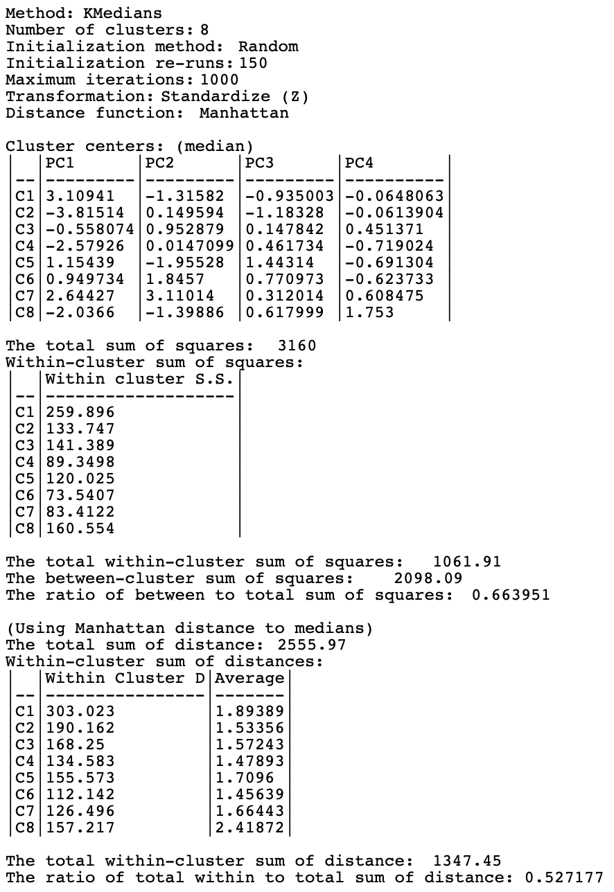
Figure 7.1: Summary - K-Medians Method, k=8

The spatial layout of the results is shown in the cluster map in Figure 7.2. The overall pattern shows great similarity with the K-Means cluster map in Figure 6.16, although the cluster sizes differ slightly. The largest cluster now consists of 160 tracts (compared to 154), and the smallest of 65 (compared to 44). While detailed cluster membership differ in minor ways, the overall pattern of where the clusters are located in the city is very similar.

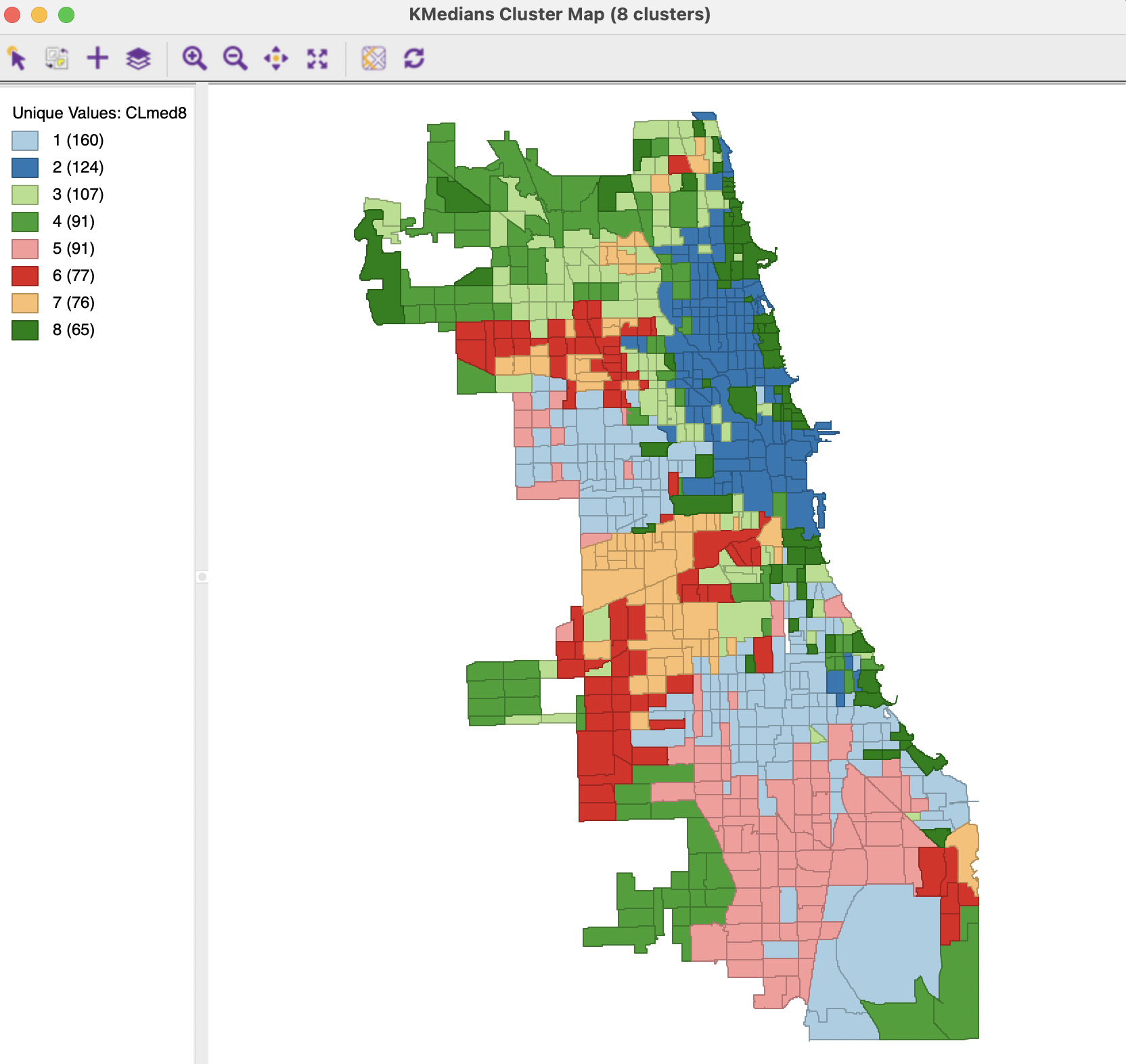
Figure 7.2: Cluster Map - K-Medians Method, k=8

7.2.2 Options and Sensitivity Analysis

K-Medians has the same options as K-Means with respect to variable transformations, maximum iterations and minimum bounds (see Section 6.3.4). KMeans++ initialization is not available, nor is the Distance Function, since only Manhattan distance is used.

As before, the cluster categories are saved as an integer variable, which can be used in other analyses.