5.4 Implementation
As mentioned in the introduction, a relatively small data set is used to illustrate the hierarchical clustering methods. The collection of socio-economic determinants of health (SDOH) for 77 Chicago Community Areas allows for a ready visualization and interpretation of the dendrogram. For larger data sets, it becomes more difficult to distinguish details in the dendrogram, although the selection of clusters by means of a cut line remains operational.
The variables in the Chicago Community Areas sample data set form a subset of the variables identified in Kolak et al. (2020) in an analysis that includes all U.S. census tracts. A subset of those census tract data will be used in the remaining chapters, for the 791 census tracts in Chicago. While not all census tract variables have a counterpart in the Chicago Community Area statistical snapshots, the match is close enough for the illustration.
Ten variables are selected:
- INCPERCAP: per capita income
- Und20: population share aged < 20
- Ov65: population share aged > 65
- Unemprt: unemployment rate
- Noveh: percentage no vehicle in the household
- Lt_high: percentage without high school education
- Rentocc: percentage renter occupied housing
- Rntburd: rent burden
- Noeng: limited English proficiency
Except for income per capita and rent burden (ratio of 12 times the median monthly rent over median income), all values are percentages computed from the original data published by the Chicago Area Metropolitan Agency for Planning (CMAP), based on 2014 American Community Survey data.
Simple descriptive statistics are provided in Figure 5.13:
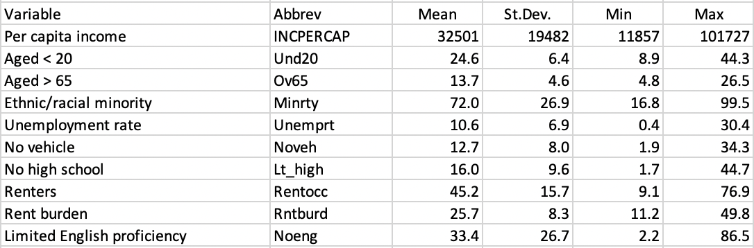
Figure 5.13: CMAP SDOH Variables Descriptive Statistics
Only per capita income and rent burden show several outlying observations at the high end. The other variables have no outliers, or only a single one (Und20, Ov65, and Lt_high).
5.4.1 Variable Settings Dialog
Hierarchical clustering is invoked from the drop down list associated with the cluster toolbar icon, as the last item in the classic clustering methods subset, shown in Figure 5.1. It can also be selected from the menu as Clusters > Hierarchical.
This brings up the Hierarchical Clustering Settings dialog, which consists of two main panels. The left panel contains the interface to specify the variables and a range of parameters, shown in Figure 5.14. The right panel provides the results, either as a Dendrogram or as a tabular Summary, each invoked by a button at the top.
In the example, the ten variables are selected, with all other items left to their default settings. This means that the initial number of clusters obtained (i.e., the location of the cut line) is set to 2, the method is Ward’s-linkage, and the variables are transformed to Standardize (Z). Since Ward’s method only works for Euclidean distance, the Distance Function is not available as an option.
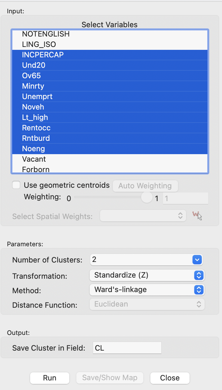
Figure 5.14: Hierarchical Clustering Variable Settings
5.4.2 Ward’s method
Clicking on the Run button generates the initial dendrogram in the right-hand panel, shown in Figure 5.15. At the very right, each observation is symbolized by a small rectangle, from which the subsequent groupings are shown as a graph. Each cluster formation is represented by a vertical line relative to the horizontal axis, with groupings closer to the right achieving a smaller total within sum of squares. As the number of clusters decreases to a manageable degree, the within sum of squares increases.
The red dashed line corresponds with the cut line, set to obtain 2 clusters (the default). The two clusters are shown with different colors for the rectangles on the right (in the illustration, light blue and dark blue). Linking and brushing is implemented, so that any subset of observations can be selected among the rectangles and identified on all the open maps and graphs.
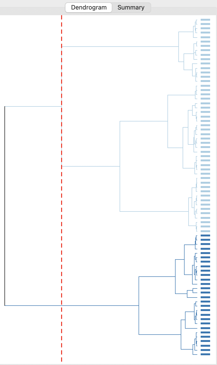
Figure 5.15: Initial Dendrogram - Ward’s Method
Typically, the initial solution is not of much interest. To obtain other cluster sizes, the cut line can be moved by grabbing it, illustrated by the highlighted pointer in Figure 5.16, for \(k\)=5. Alternatively, the Number of Clusters can also be changed in the dialog, which automatically will move the cut line to the corresponding location and adjust the cluster groupings of the individual observations.
In Figure 5.16, the result is shown for \(k\)=5.
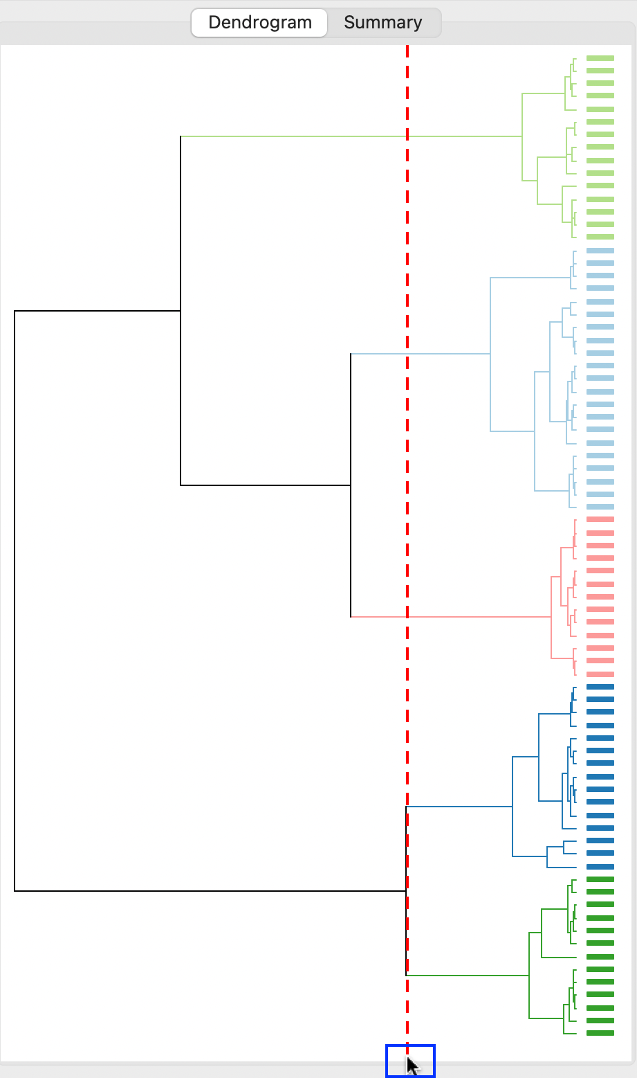
Figure 5.16: Dendrogram - Ward’s Method, k=5
At this point, invoking Save/Show Map has three direct results: the cluster classification is saved in the data table using the variable name specified in Save Cluster in Field (in the example, this is set to CLward); the Summary table becomes available; and a Cluster Map is produced as a unique values map with the cluster classifications.
As mentioned, the classification labels are meaningless. The convention used in GeoDa is to label the largest cluster as 1 with subsequent labels in decreasing order of size.
The summary table in the example is shown in Figure 5.17, with the corresponding cluster map in Figure 5.18.
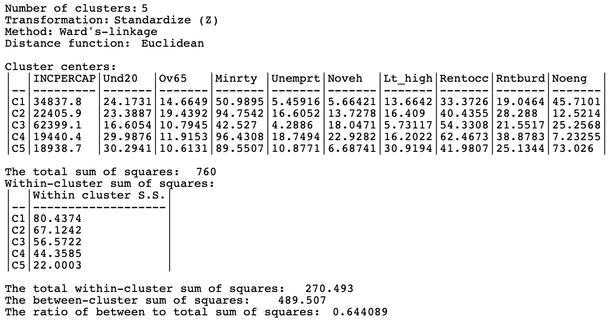
Figure 5.17: Summary - Ward’s Method, k=5
For each cluster, the cluster centers are given as the average for that variable computed from the observations in the cluster.28 This allows for a substantive interpretation, although that is not always straightforward. For example, cluster 3 (C3) achieves the highest value for income per capita, and the lowest entries for under 20, percent minority, unemployment rate, and less than high school. This would suggest a higher income cluster, but it has the second highest value of absence of cars and percent renters, and the third of percent not English speaking. Clearly, the interpretation and labeling of the resulting clusters requires some creativity and imagination.
Below the cluster centers follows The total sum of squares, which here is 760, with the Within-cluster sum of squares listed for each cluster.29 At the bottom of the summary are the overall statistics, including the total within-cluster sum of squares, at 270.493 (the sum of the individual cluster entries), the between-cluster sum of squares, at 489.507, and the ratio of between to total sum of squares, at 0.644089. A higher ratio indicates better cluster performance.
A useful option is to Save the cluster results to a text file. This is selected by right clicking on the panel.
The cluster map depicts the location of the cluster members and the cardinality of each cluster. This is a way to spatialize the outcome of an otherwise non-spatial clustering method.
The largest cluster contains 21 community areas, followed by two clusters with 15 and two with 13 members. In this example, the clusters are also fairly spatially compact, with cluster 3 consisting largely of community areas in the north-east of the city, except for two community areas (Kenwood and Hyde Park) that form a small enclave surrounded by cluster 4. The latter is characterized by a high percentage minority, high unemployment and rent burden, in stark contrast with the characteristics of cluster 3.
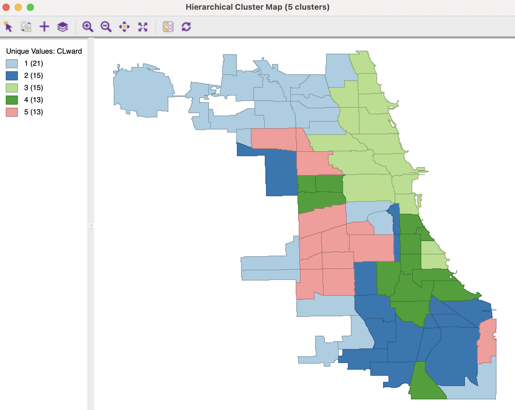
Figure 5.18: Cluster Map - Ward’s Method, k=5
Setting the number of clusters at five is by no means necessarily the best solution. In an actual application of hierarchical clustering, one would experiment with different cut points and evaluate the solutions.
For completeness sake, the dendrogram, summary and cluster maps are shown next for the three other linkage methods.
5.4.3 Single linkage
The linkage options are chosen from the Method item in the dialog. The cluster results for single linkage are typically characterized by one or a few very large clusters and several singletons (one observation per cluster). This characteristic is confirmed in the example, with the dendrogram shown in Figure 5.19, for \(k\)=5. The graph indicates how all but four observations are grouped into a single cluster. This situation is not remedied by moving the cut point such that more clusters result, since almost all of the additional clusters are singletons as well.
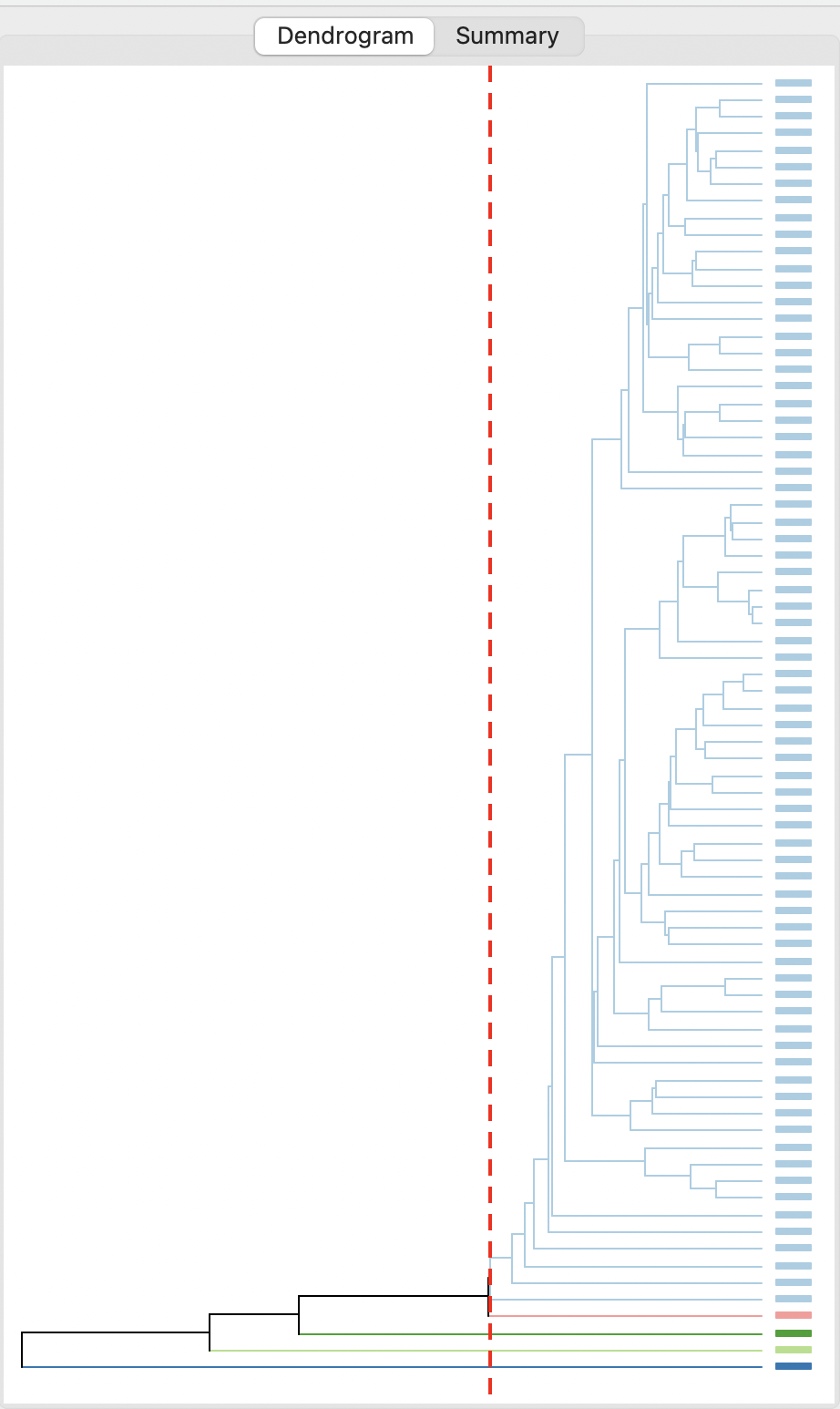
Figure 5.19: Dendrogram - Single Linkage, k=5
The summary in Figure 5.20 lists a within cluster sum of squares of zero for the four singletons. The overall fit is poor, with a between to total ratio of only 0.120291.
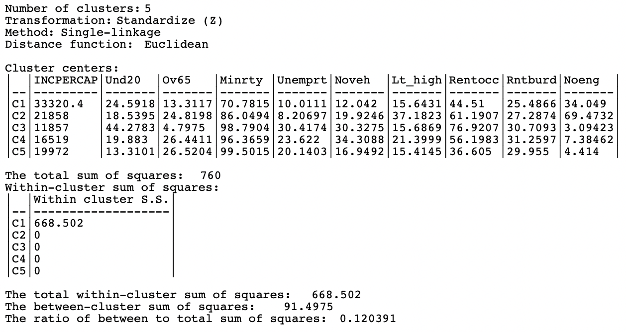
Figure 5.20: Summary - Single Linkage, k=5
The cluster map in Figure 5.21 highlights the four outliers. In other respects, this map is uninteresting, given the large size of the dominant cluster.
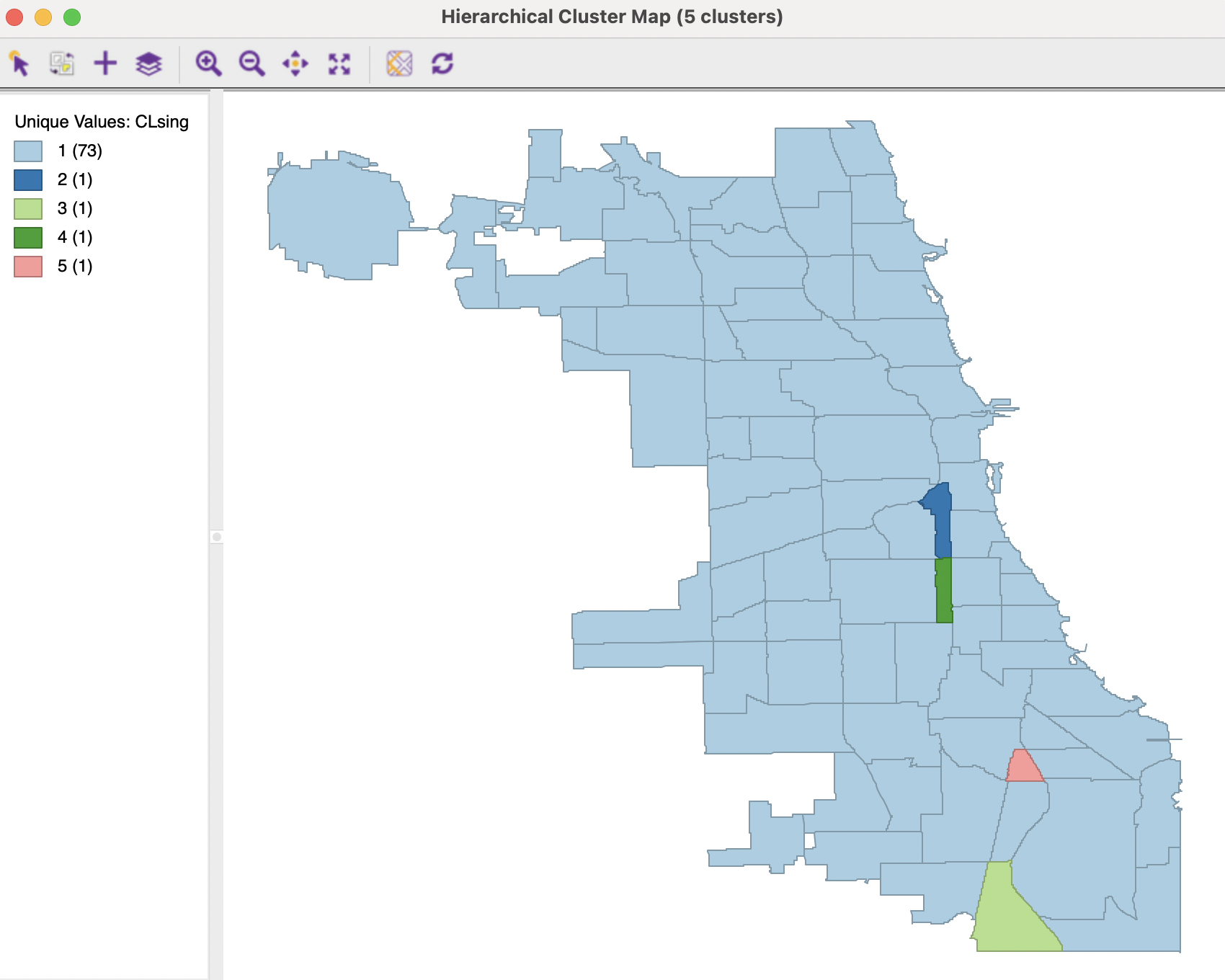
Figure 5.21: Cluster Map - Single Linkage, k=5
In practice, in most situations, single linkage will not be a good choice, unless the objective is to identify a lot of singletons and characterize these as outliers.
5.4.4 Complete linkage
The complete linkage method yields clusters that are similar in balance to Ward’s method. For example, in Figure 5.22, the dendrogram is shown, using a cut point with five clusters. While much more balanced than single linkage, the smallest clusters are much smaller than the others.
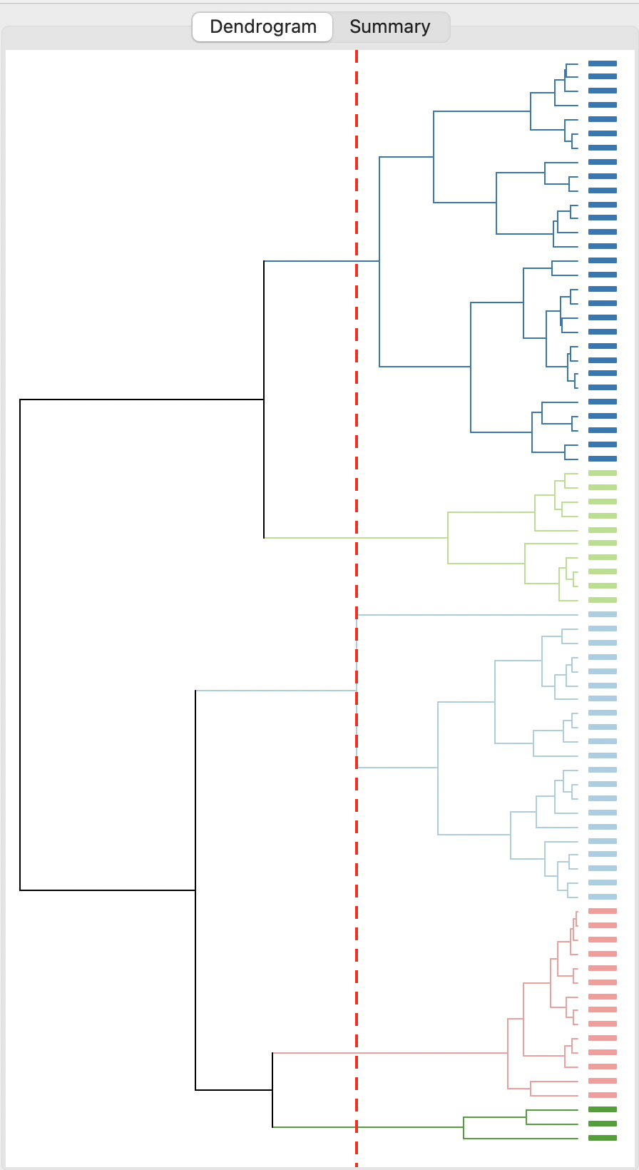
Figure 5.22: Dendrogram - Complete Linkage, k=5
The summary in Figure 5.23 reveals performance similar but slightly inferior to Ward’s method. The ratio of between to total is 0.600629, compared to 0.644089 for Ward’s method.
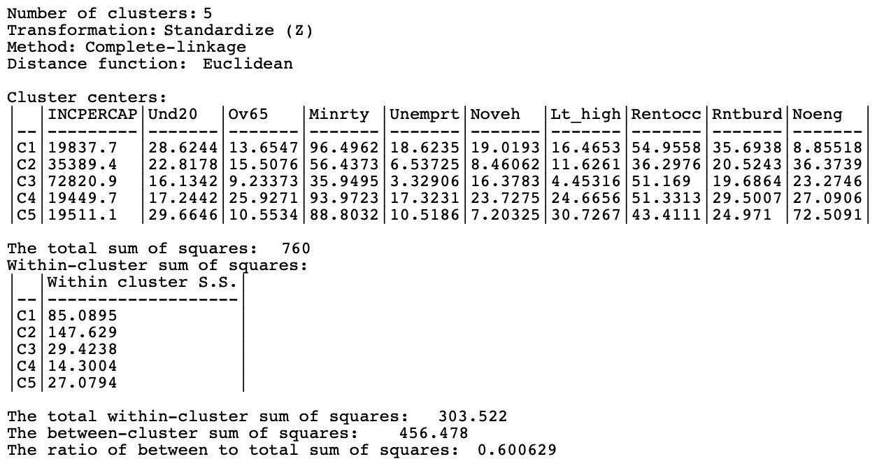
Figure 5.23: Summary - Complete Linkage, k=5
The cluster map in Figure 5.24 shows how several of the previously identified outliers are now grouped in cluster 5. The overall spatial layout is similar to that obtained for Ward’s method, although the cluster sizes are different.
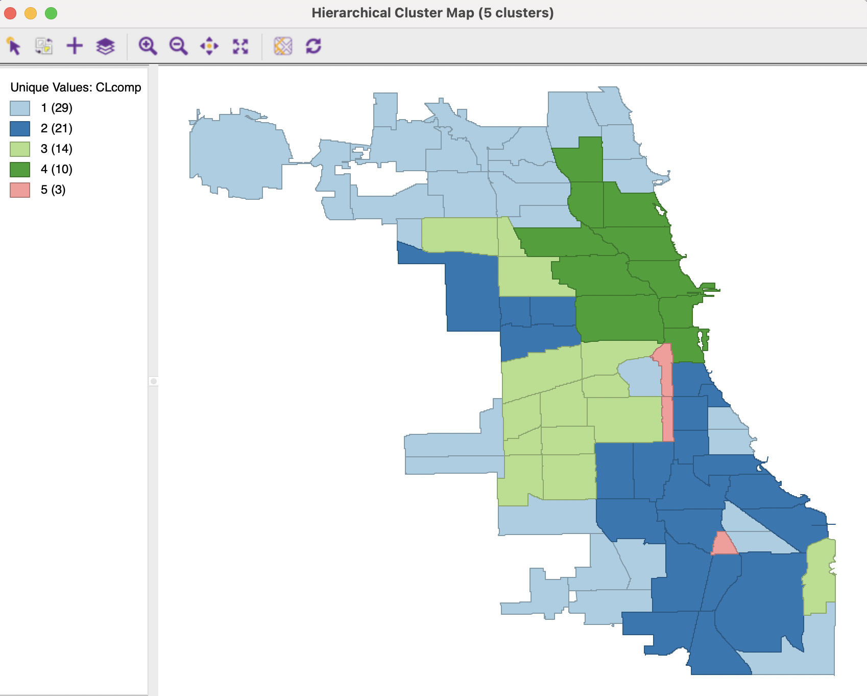
Figure 5.24: Cluster Map - Complete Linkage, k=5
5.4.5 Average linkage
Finally, the average linkage criterion suffers from some of the same problems as single linkage, although it yields slightly better results. The dendrogram in Figure 5.25 indicates a somewhat unbalanced structure, with two singletons and two clusters much larger than the third.
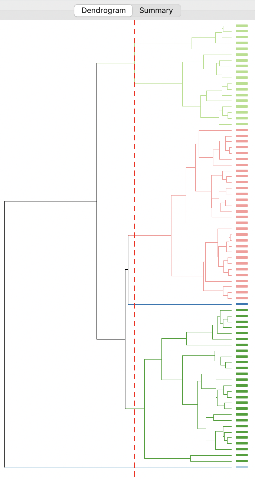
Figure 5.25: Dendrogram - Average Linkage, k=5
As given in Figure 5.26, the summary characteristics are better than in the single linkage case, with only two singletons. However, the overall ratio of between to total sum of squares is still considerably inferior to Ward’s and complete linkage, at 0.522972.
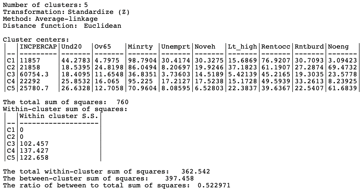
Figure 5.26: Summary - Average Linkage, k=5
The cluster map in Figure 5.27 again identifies two of the outliers from the single linkage map as singletons, but the others are absorbed into the larger clusters.
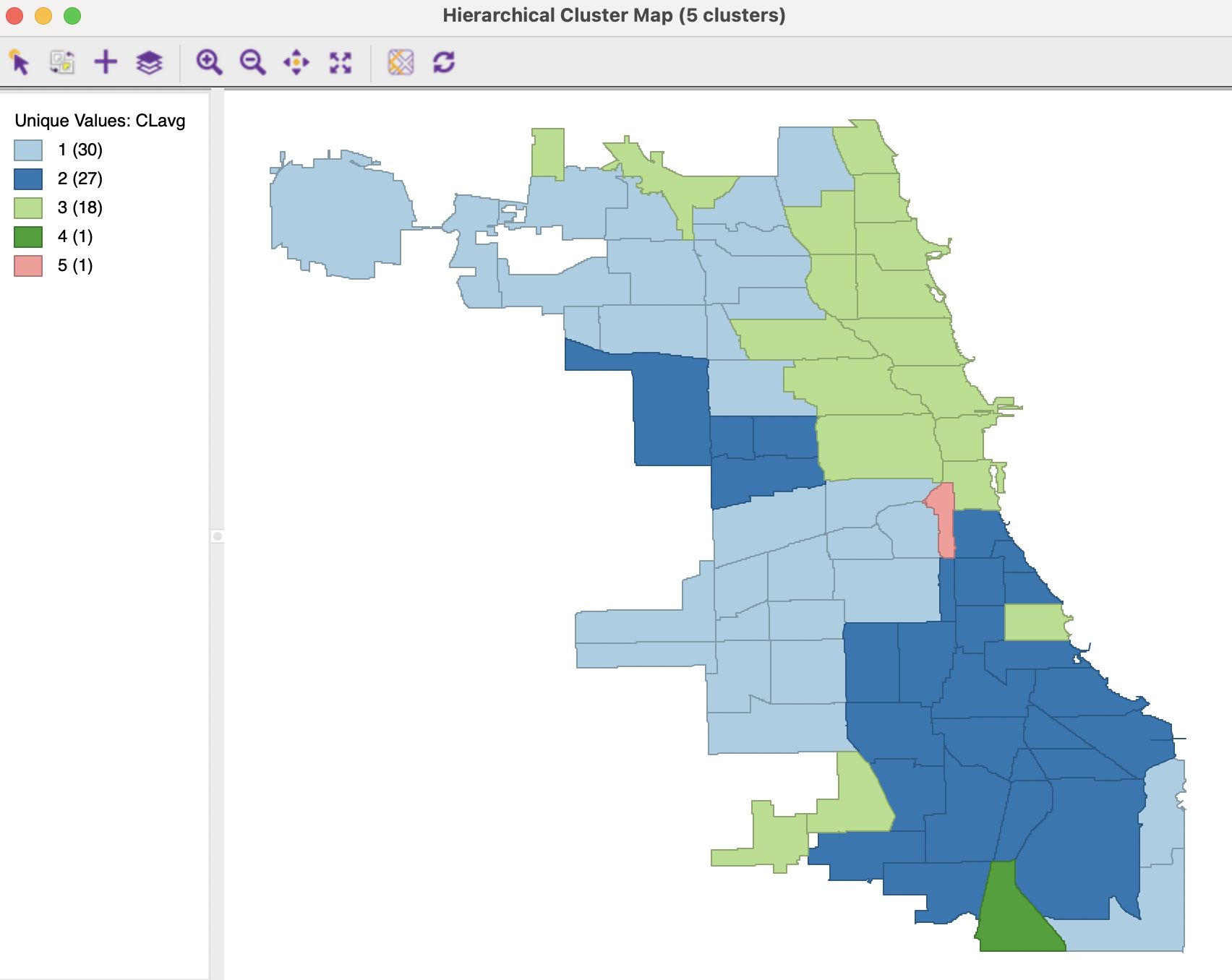
Figure 5.27: Cluster Map - Average Linkage, k=5
5.4.6 Sensitivity Analysis
Many parameters can be altered to assess the sensitivity of the cluster solution. This does not only pertain to the number of clusters (\(k\)) and the linkage method, but also to the distance metric, and, to a lesser extent, to the transformation.
The advantage of hierarchical clustering is that it is straightforward to change the number of clusters and assess the effect on cluster characteristics and spatial layout. As mentioned, a drawback is that observations are locked into a particular branch of the dendrogram, which limits the flexibility of later grouping.
The resulting clusters can be exploited in a number of different data analyses, which is pursued further in the next chapter.