7.3 K-Medoids

The objective of the K-Medoids algorithm is to minimize the sum of the distances from the observations in each cluster to a representative center for that cluster. In contrast to K-Means and K-Medians, the cluster centers are actual observations and thus do not need to be computed separately (as mean or median).

K-Medoids works with any dissimilarity matrix, since it only relies on inter-observation distances and does not require a mean or median center. When actual observations are available, the Manhattan distance is the preferred metric, since it is less affected by outliers. In addition, since the objective function is based on the sum of the actual distances instead of their squares, the influence of outliers is even smaller.³⁴

The objective function is expressed as finding the cluster assignments \(C(i)\) such that, for a given \(k\): \[\mbox{argmin}_{C(i)} \sum_{h=1}^k \sum_{i \in h} d_{i,h_c},\] where \(h_c\) is a representative center for cluster \(h\) and \(d\) is the distance metric used (from a dissimilarity matrix). As was the case for K-Means (and K-Medians), the problem is NP hard and an exact solution does not exist.

The K-Medoids objective is identical in structure to that of a simple (unweighted) location-allocation facility location problem. Such problems consist of finding \(k\) optimal locations among \(n\) possibilities (the location part), and subsequently assigning the remaining observations to those centers (the allocation part).³⁵

The main approach to solve the K-Medoids problem is the so-called partitioning around medoids (PAM) algorithm of Kaufman and Rousseeuw (2005). The logic underlying the PAM algorithm involves two stages, labeled BUILD and SWAP.

7.3.1 The PAM Algorithm for K-Medoids

In the BUILD stage, a set of \(k\) starting centers are selected from the \(n\) observations. In some implementations, this is a random selection, but Kaufman and Rousseeuw (2005), and, more recently Schubert and Rousseeuw (2019) prefer a step-wise procedure that optimizes the initial set.

The main part of the algorithm consists of the SWAP stage. This proceeds in a greedy iterative manner by swapping a current center with a candidate from the remaining non-centers, as long as the objective function can be improved.³⁶

7.3.1.1 Build

The BUILD phase of the algorithm consists of identifying \(k\) observations out of the \(n\) and assigning them to be cluster centers \(h\), with \(h = 1, \dots, k\). Kaufman and Rousseeuw (2005) outline a step-wise approach that starts by picking the center, say \(h_1\), that minimizes the overall sum of distances. This is readily accomplished by taking the observation that corresponds with the smallest row sum (or, equivalently, column sum) of the dissimilarity matrix.

The algorithm is again illustrated with the same toy example used in the previous two chapters. This consists of the seven point coordinates listed in Figure 6.3, with \(k=2\) as the number of clusters. The corresponding Manhattan inter-point distance matrix is given in Figure 7.3. The row sums for each observation, are, respectively: 43, 32, 27, 24, 25, 37, and 33. The lowest value (24) is obtained for point 4, i.e., (6, 6), which is selected as the first cluster center.

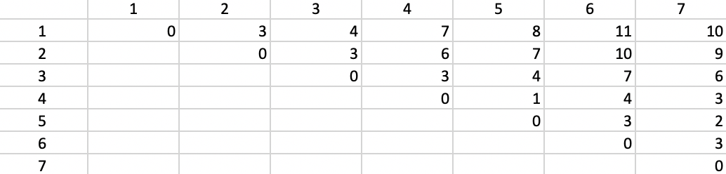
Figure 7.3: Manhattan Inter-Point Distance Matrix

Next, at each step, an additional center (for \(h = 2, \dots, k\)) is selected that improves the objective function the most. This is accomplished by evaluating each of the remaining points as a potential center. The one is selected that results in the greatest reduction in the objective function.

With the first center assigned, a \((n-1) \times (n-1)\) submatrix of the original distance matrix is used to assess each of the remaining \(n-1\) points (i.e., not including \(h_1\)) as a potential new center. This is implemented by computing the improvement that would result for each column point \(j\) from selecting a given row \(i\) as the new center. The row (destination) for with the improvement over all columns (origins) is largest is selected as the new center.

More specifically, in the second iteration the current distance between the point in column \(j\) and \(h_1\) is compared to the distance from \(j\) to each row \(i\). If \(j\) is closer to \(i\) than to its current closest center, then \(d_{j,h_1} - d_{ji} > 0\), the potential improvement from assigning \(j\) to center \(i\) instead of to its current closest center. In the second iteration, this is \(h_1\), but in later iterations it is more generally the closest center. Negative entries are not taken into account.

The row \(i\) for which the sum of the improvements over all \(j\) is the greatest becomes the next center. In the example, with point 4 as the first center, its distance from each of the remaining six points is listed in the second row of Figure 7.4, below the label of the point. Each of the following rows in the table gives the improvement in distance from the point at the top if the row point were selected as the new center, or \(\mbox{max}(d_{j4} - d_{ij},0)\). For example, for row 1 and column 2, that value is \(6 - d_{1,2} = 6 - 3 = 3\). For the other points (columns), the point 4 is closer than 2, so the corresponding matrix entries are zero, resulting in an overall row sum of 3 (the improvement in the objective from selecting 2 as the next center).

The row sum for each potential center is given in the column labeled sum. There is a tie between observations 3 and 7, which each achieve an improvement of 6. For consistency with the earlier chapters, point 7 is selected as the second starting point.

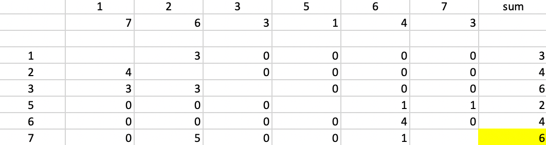
Figure 7.4: BUILD - Step 2

At this stage, the distance for each \(j\) to its nearest center is updated and the process starts anew for the \(n-2\) remaining observations. This process continues until all \(k\) centers have been assigned. This provides the initial solution for the SWAP stage. Since the example only has \(k=2\), the two initial centers are points 4 and 7.

7.3.1.2 Swap

All the observations are assigned to the cluster center they are closest to. As shown in Figure 7.5, this results in cluster 1 consisting of observations 1-5, and cluster 2 being made up of observations 6 and 7, using the distances from columns 4 and 7 in the dissimilarity matrix. The total distance to each cluster center equals 20, with cluster 1 contributing 17 and cluster 2, 3

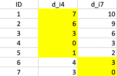
Figure 7.5: Cluster Assignment at end of BUILD stage

The essence of the SWAP phase is to consider what happens to the overall objective when a current center (one of the \(k\)) is swapped with one of the remaining \(n - k\) non-centers. With a current center labeled as \(i\) and a non-center as \(r\), this requires the evaluation of \(k \times (n-k)\) possible swaps (\(i, r\)).

When considering the effect of replacing a center \(i\) by a new center \(r\), the impact on all the remaining \(n - k -1\) points must be considered. Those points can no longer be assigned to \(i\), so they either become part of a cluster around the new center \(r\), or they are re-allocated to one of the other centers \(g\) (but not \(i\), since that is no longer a center).

For each point \(j\), the change in distance associated with a swap \((i, r)\) is labeled as \(C_{jir}\). The total improvement for a given swap \((i, r)\) is the sum of its effect over all \(j\), \(T_{ir} = \sum_j C_{jir}\). This total effect is evaluated for all possible \((i, r)\) pairs and the minimum is selected. If that minimum is also negative, the associated swap is carried out, i.e., when \(\mbox{argmin}_{i,r} T_{ir} < 0\), \(r\) takes the place of \(i\).

This process is continued until no more swaps can achieve an improvement in the objective function. The computational burden associated with this algorithm is quite high, since at each iteration \(k \times (n - k)\) pairs need to be evaluated. On the other hand, no calculations other than comparison and addition/subtraction are involved, and all the information is in the (constant) dissimilarity matrix.

To compute the net change in the objective function for a point \(j\) that follows from a swap between \(i\) and \(r\), two cases can be distinguished. In one, \(j\) was not assigned to center \(i\), but it belongs to a different cluster, say \(g\), such that \(d_{jg} < d_{ji}\). In the other case, \(j\) does initially belong to the cluster \(i\), such that \(d_{ji} < d_{jg}\) for all other centers \(g\). In both instances, the distances from \(j\) to the nearest current center (\(i\) or \(g\)) must be compared to the distance to the candidate point, \(r\).

The first instance, where \(j\) is not part of the cluster \(i\) is illustrated in Figure 7.6. There are two scenarios for the configuration of the point \(j\), labeled \(j1\) and \(j2\). Both these points are closer to \(g\) than to \(i\), since they are not part of the cluster around \(i\).

The key element is whether \(j\) is closer to \(r\) than to its current cluster center \(g\). If \(d_{jg} \le d_{jr}\), then nothing changes, since \(j\) remains in cluster \(g\), and \(C_{jir} = 0\). This is the case for point \(j1\). The dashed red line gives the distance to the current center \(g\) and the dashed green line gives the distance to \(r\).

If \(j\) is closer to the new center \(r\) than to its current cluster \(g\), then \(d_{jr} < d_{jg}\), as is the case for point \(j2\). As a result, \(j\) is assigned to the new center \(r\) and \(C_{jir} = d_{jr} - d_{jg}\), a negative value, which decreases the overall cost. In the figure, the length of the dashed red line must be compared to the length of the solid green line, which designates a re-assignment of \(j\) to the candidate center \(r\).

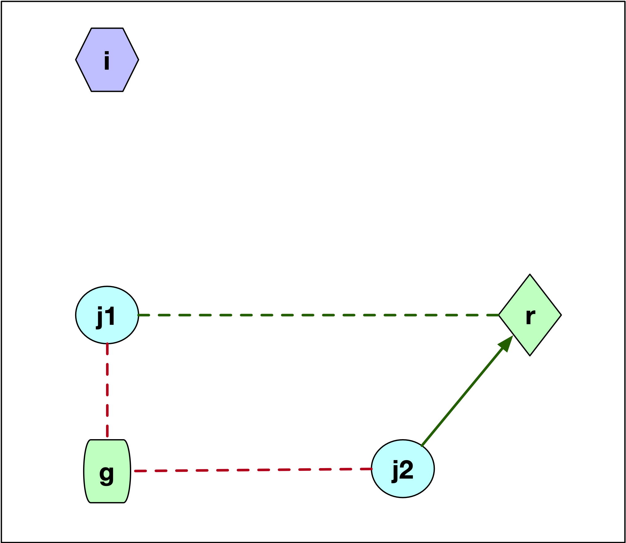
Figure 7.6: PAM SWAP Point Layout - Case 1

The second configuration is shown in Figure 7.7, where \(j\) starts out as being assigned to \(i\). There are three possibilities for the location of \(j\) relative to \(g\) and \(r\). In the first case, illustrated by point \(j1\), \(j\) is closer to \(g\) than to \(r\). This is illustrated by the difference in length between the dashed green line (\(d_{j1r}\)) and the solid green line (\(d_{j1g}\)). More precisely, \(d_{jr} \geq d_{jg}\) so that \(j\) is now assigned to \(g\). The change in the objective is \(C_{jir} = d_{jg} - d_{ji}\). This value is positive, since \(j\) was part of cluster \(i\) and thus was closer to \(i\) than to \(g\) (compare the length of the red dashed line between \(j1\) and \(i\) and the length of the line connecting \(j1\) to \(g\)).

If \(j\) is closer to \(r\), then \(d_{jr} < d_{jg}\). There are two possible layouts, one depicted by \(j2\), the other by \(j3\). In both instances, the result is that \(j\) is assigned to \(r\), but the effect on the objective differs.

In the Figure, for both \(j2\) and \(j3\) the dashed green line to \(g\) is longer than the solid green line to \(r\). The change in the objective is the difference between the new distance and the old one (\(d_{ji}\)), or \(C_{jir} = d_{jr} - d_{ji}\). This value could be either positive or negative, since what matters is that \(j\) is closer to \(r\) than to \(g\), irrespective of how close \(j\) might have been to \(i\). For point \(j2\), the distance to \(i\) (dashed red line) was smaller than the new distance to \(r\) (solid green line), so \(d_{jr} - d_{ji} > 0\). In the case of \(j3\), the opposite holds, and the length to \(i\) (dashed red line) is larger than the distance to the new center (solid green line). In this case, the change to the objective is \(d_{jr} - d_{ji} < 0\).

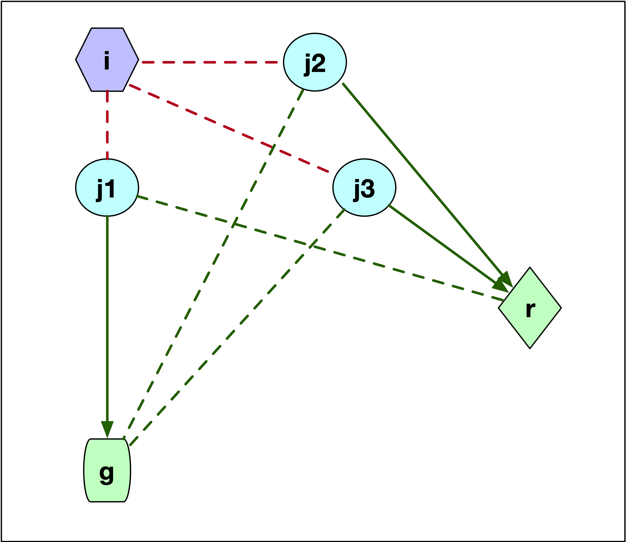
Figure 7.7: PAM SWAP Point Layout - Case 2

In the example, the first step in the swap procedure consists of evaluating whether center 4 or center 7 can be replaced by any of the current non-centers, i.e., 1, 2, 3, 5, or 6. The comparison involves three distances for each point: the distance to the closest center, the distance to the second closest center, and the distance to the candidate center. In the toy example, this is greatly simplified, since there are only two centers, with distances \(d_{j4}\) and \(d_{j7}\) for each non-candidate and non-center point \(j\). In addition, the distance to the candidate center \(d_{jr}\) is needed, where each non-center point is in turn considered as a candidate (\(r\)).

All the evaluations for the first step are included in Figure 7.8. There are five main panels, one for each current non-center point. The rows in each panel are the non-center, non-candidate points. For example, in the top panel, 1 is considered a candidate, so the rows pertain to 2, 3, 5, and 6. Columns 3-4 give the distance to, respectively, center 4 (\(d_{j4}\)), center 7 (\(d_{j7}\)) and candidate center 1 (\(d_{j1}\)).

Columns 5 and 6 give the contribution of each row to the objective with point 1 replacing, respectively 4 (\(C_{j41}\)) and 7 (\(C_{j71}\)). In the scenario of replacing point 4 by point 1, the distances from point 2 to 4 and 7 are 6 and 9, so point 2 is closest to center 4. As a result 2 will be allocated to either the new candidate center 1 or the current center 7. It is closest to the new center (distance 3 relative to 9). The decrease in the objective from assigning 2 to 1 rather than 4 is 3 - 6 = -3, the entry in the column \(C_{j41}\).

Identical calculations are carried out to compute the contribution of 2 to the replacement of 7 by 1. Since 2 is closer to 4, this is the situation where a point is not closest to the center that is to be replaced. The assessment is whether point 2 would stay with its current center (4) or move to the candidate. Since 2 is closer to 1 than to 4, the gain from the swap is again -3, entered under \(C_{j71}\). In the same way, the contributions are computed for each of the other non-center and non-candidate points. The sum of the contributions is listed in the row labeled \(T\). For a replacement of 4 by 1, the sum of -3, 1, 1, and 0 gives -1 as the value of \(T_{41}\). Similarly, the value of \(T_{47}\) is the sum of -3, 0, 0, and 1, or -2.

The remaining panels show the results when each of the other current non-centers is evaluated as a center candidate. The minimum value over all pairs \(i,r\) is obtained for \(T_{43} = -5\). This suggests that center 4 should be replaced by point 3 (there is actually a tie with \(T_{73}\), so in each case 3 should enter the center set; in the example, it replaces 4). The improvement in the overall objective function from this step is -5.

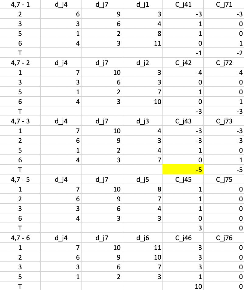
Figure 7.8: PAM SWAP Cost Changes - Step 1

This process is repeated in Figure 7.9, but now using \(d_{j3}\) and \(d_{j7}\) as reference distances. The smallest value for \(T\) is found for \(T_{75} = -2\), which is also the improvement to the objective function (note that the improvement is smaller than for the first step, something that is to be expected from a gradient descent method). This suggests that 7 should be replaced by 5.

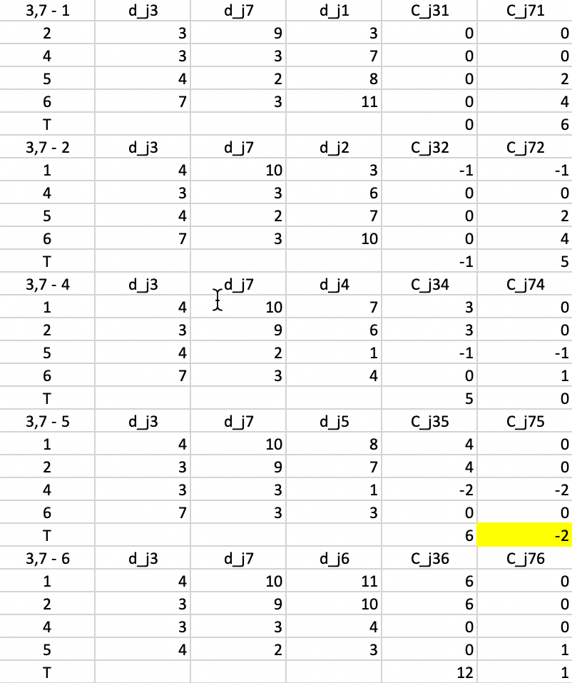
Figure 7.9: PAM SWAP Cost Changes - Step 2

In the next step, shown in Figure 7.10, the calculations are repeated, using \(d_{j3}\) and \(d_{j5}\) as the distances. The smallest value for \(T\) is found for \(T_{32} = -1\), suggesting that 3 should be replaced by 2. The improvement in the objective is -1 (again, smaller than in the previous step).

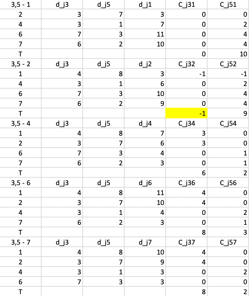
Figure 7.10: PAM SWAP Cost Changes - Step 3

In the last step, shown in Figure 7.11, everything is recalculated for \(d_{j2}\) and \(d_{j5}\). At this stage, none of the \(T\) yield a negative value, so the algorithm has reached a local optimum and stops.

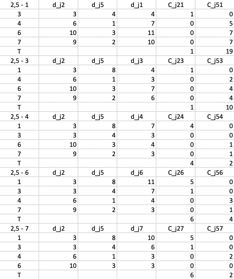
Figure 7.11: PAM SWAP Cost Changes - Step 4

The final result consists of a cluster of three elements, with observations 1 and 3 centered on 2, and a cluster of four elements, with observations 4, 6 and 7 centered on 5. As Figure 7.12 illustrates, both clusters contribute 6 to the total sum of deviations, for a final value of 12. This also turns out to be 20 - 5 - 2 - 1, or the total effect of each swap on the objective function.

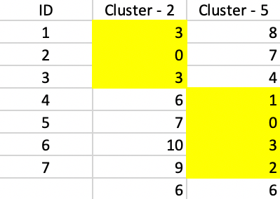
Figure 7.12: PAM SWAP Final Assignment

7.3.2 Improving on the PAM Algorithm

The complexity of each iteration in the original PAM algorithm is of the order \(k \times (n - k)^2\), which means it will not scale well to large data sets with potentially large values of \(k\). To address this issue, several refinements have been proposed. The most familiar ones are CLARA, CLARANS and LAB.

7.3.2.1 CLARA

Kaufman and Rousseeuw (2005) proposed the algorithm CLARA, based on a sampling strategy. Instead of considering the full data set, a subsample is drawn. Then the PAM algorithm is applied to find the best \(k\) medoids in the sample. Finally, the distance from all observations (not just those in the sample) to their closest medoid is computed to assess the overall quality of the clustering.

The sampling process can be repeated for several more samples (keeping the best solution from the previous iteration as part of the sampled observations), and at the end the best solution is selected. While easy to implement, this approach does not guarantee that the best local optimum solution is found. In fact, if one of the best medoids is never sampled, it is impossible for it to become part of the final solution. Note that as the size of the sample becomes closer to the size of the full data set, the results will tend to be similar to those given by PAM.³⁷

In practical applications, Kaufman and Rousseeuw (2005) suggest to use a sample size of 40 + 2k and to repeat the process 5 times.³⁸

7.3.2.2 CLARANS

In Ng and Han (2002), a different sampling strategy is outlined that keeps the full set of observations under consideration. The problem is formulated as finding the best node in a graph that consists of all possible combinations of \(k\) observations that could serve as the \(k\) medoids. The nodes are connected by edges to the \(k \times (n - k)\) nodes that differ in one medoid (i.e., for each edge, one of the \(k\) medoid nodes is swapped with one of the \(n - k\) candidates).

The algorithm CLARANS starts an iteration by randomly picking a node (i.e., a set of \(k\) candidate medoids). Then, it randomly picks a neighbor of this node in the graph. This is a set of \(k\) medoids where one is swapped with the current set. If this leads to an improvement in the cost, then the new node becomes the new start of the next set of searches (still part of the same iteration). If not, another neighbor is picked and evaluated, up to maxneighbor times. This ends an iteration.

At the end of the iteration the cost of the last solution is compared to the stored current best. If the new solution constitutes an improvement, it becomes the new best. This search process is carried out a total of numlocal iterations and at the end the best overall solution is kept. Because of the special nature of the graph, not that many steps are required to achieve a local minimum (technically, there are many paths that lead to the local minimum, even when starting at a random node).

Again, this can be illustrated by means of the toy example. To construct \(k=2\) clusters, any pair of 2 observations from the 7 could be considered a potential medoid. All those pairs constitute the nodes in the graph. The total number of nodes is given by the binomial coefficient \({n}\choose{k}\). In the example, \({{7}\choose{2}} = 21\).

Each of the 21 nodes in the graph has \(k \times (n - k) = 2 \times 5 = 10\) neighbors that differ only in one medoid connected with an edge. For example, the initial node corresponding to (4,7) will be connected to all the nodes that differ by one medoid, i.e., either 4 or 7 is replaced (swapped in PAM terminology) by one of the \(n - k = 5\) remaining nodes. Specifically, this includes the following 10 neighbors: 1-7, 2-7, 3-7, 5-7, 6-7, and 4-1, 4-2, 4-3, 4-5 and 4-6. Rather than evaluating all 10 potential swaps, as in PAM, only a maximum number (maxneighbor) are evaluated. At the end of those evaluations, the best solution is kept. Then the process is repeated, up to the specified total number of iterations, which Ng and Han (2002) call numlocal.

With maxneighbors set to 2, the first step of the random evaluation could be to randomly pick the pair 4-5 from the neighboring nodes. In other words, 7 in the original set is replaced by 5. Using the values from the worked example above, we have \(T_{45} = 3\), a positive value, so this does not improve the objective function. The iteration count is increased (for maxneighbors) and a second random node is picked, e.g., 4-2 (i.e., replacing 7 by 2). At this stage, the value \(T_{42} = -3\), so the objective is improved to 20-3 = 17. Since the end of maxneighbors has been reached, this value is stored as best and the process is repeated with a different random starting point. This is continued until numlocal local optima have been obtained. At that point, the best overall solution is kept.

Based on several numerical experiments, Ng and Han (2002) suggest that no more than 2 iterations need to be pursued (i.e., numlocal = 2), with some evidence that more operations are not cost-effective. They also suggest a sample size of 1.25% of \(k \times (n-k)\).³⁹

Both CLARA and CLARANS are large data methods, since for smaller data sizes (e.g., \(n < 100\)), PAM will be feasible and obtain better solutions (since it implements an exhaustive evaluation).

Further speedup of PAM, CLARA and CLARANS is outlined in Schubert and Rousseeuw (2019), where some redundancies in the comparison of distances in the SWAP phase are removed. In essence, this exploits the fact that observations allocated to a medoid that will be swapped out, will move to either the second closest medoid or to the swap point. Observations that are not currently allocated to the medoid under consideration will either stay in their current cluster, or move to the swap point, depending on how the distance to their cluster center compares to the distance to the swap point. These ideas shorten the number of loops that need to be evaluated and allow the algorithms to scale to much larger problems (details are in Schubert and Rousseeuw 2019, 175). In addition, they provide and option to carry out the swaps for all current k medoids simultaneously, similar to the logic in K-Means, implemented in the FASTPAM2 algorithm (see Schubert and Rousseeuw 2019, 178).

7.3.2.3 LAB

A second type of improvement in the algorithm pertains to the BUILD phase. The original approach is replaced by a so-called Linear Approximative BUILD (LAB), which achieves linear runtime in \(n\). Instead of considering all candidate points, only a subsample from the data is used, repeated \(k\) times (once for each medoid).

The FastPAM2 algorithm tends to yield the best cluster results relative to the other methods, in terms of the smallest sum of distances to the respective medoids. However, especially for large \(n\) and large \(k\), FastCLARANS yields much smaller compute times, although the quality of the clusters is not as good as for FastPAM2. FastCLARA is always much slower than the other two. In terms of the initialization methods, LAB tends to be much faster than BUILD, especially for larger \(n\) and \(k\).

7.3.3 Implementation

K-Medoids clustering is invoked from the drop down list associated with the cluster toolbar icon, as the third item in the classic clustering methods subset, part of the full list shown in Figure 6.1. It can also be selected from the menu as Clusters > K Medoids.

This brings up the KMedoids Clustering Settings dialog. This dialog has an almost identical structure to the one for K-Medians, with a left hand panel to select the variables and specify the cluster parameters, and a right hand panel that lists the Summary results.

The method is illustrated with the Chicago SDOH sample data set. However, unlike the examples for K-Means and K-Medians, the variables selected are the X and Y coordinates of the census tracts. This showcases the location-allocation aspect of the K-Medoids method.

In the variable selection interface, the drop down list contains <X-Centroids> and <Y-Centroids> as available variables, even when those coordinates have not been computed explicitly. They are included to facilitate the implementation of the spatially constrained clustering methods in Part III. The data layer is projected, with the coordinates expressed in feet, which makes for rather large numbers.

The default setup is to use the Standardize (Z) transformation, with the FastPAM algorithm using the LAB initialization. The distance function is set to Manhattan. As before, the number of clusters is chosen as 8. There are no other options to be set, since the PAM algorithm proceeds with an exhaustive search in the SWAP phase, after the initial \(k\) medoids are selected.

Invoking Run populates the Summary panel with properties of the cluster solution and brings up a separate window with the cluster map. The cluster classification are saved as an integer variable with the specified Field name.

7.3.3.1 Cluster results

The cluster characteristics are shown in Figure 7.13. Below the usual listing of methods and options, the observation numbers of the eight cluster medoids are given. These can be used to select the corresponding observations in the table. As before, the values for the different variables in each cluster center are listed, but now these correspond to actual observations. However, in the current application, the X and Y centroids are not part of the data table, unless they were added explicitly.

The customary sum of squares measures are included for completeness, but as pointed out in the discussion of K-Medians, these do not match the criteria used in the objective function. Nevertheless, the BSS/TSS ratio of 0.870416 shows a good separation between the eight clusters. Since the mean of the coordinates is close to the centroid, this ratio is actually not a totally inappropriate metric. However, in contrast to the objective function used, the distances are Euclidean and not Manhattan block distances.

The latter are employed in the calculation of the within-cluster sum of distances. As for K-Medians, both the total distance per cluster as well as the average are listed. The most compact cluster is C8, with an average distance of 0.413. The least compact cluster is C6, with an average of 0.745, closely followed by C2 (0.702). The ratio of within to total sum of the distances indicates a significant reduction to 0.34 of the original.

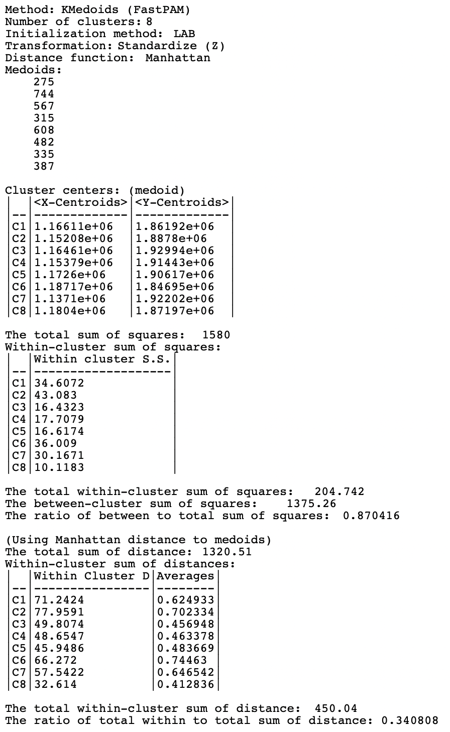
Figure 7.13: Summary, K-Medoids, k=8

The spatial layout of the clusters is shown in the cluster map in Figure 7.14. In addition to the cluster membership for each tract, the cluster centers (medoid) are highlighted in black on the map. These are shown as tract polygons, although the actual cluster exercise was carried out for the tract centroids (points).⁴⁰

The clusters show the optimal allocation of the 791 census tracts to 8 centers. The result is the most balanced of the cluster groupings obtained so far, with the four largest clusters consisting of between 114 and 105 tracts, and the four smallest between 95 and 79. In addition, the clusters are almost perfectly spatially contiguous, even though K-Medoids is a non-spatial clustering method. This illustrates the application of standard clustering methods to location coordinates to delineate regions in space, a topic that is revisited in Chapter 9.

The one outlier tract that belongs to cluster 2 may seem to be a mistake, since it seems closer to the center of cluster 1 than to that of cluster 2, to which it has been assigned. However, the distances used in the algorithm are not straight line, but Manhattan distances. This case involves an instance where the centroid of the tract involved is almost directly south of the cluster 2 center, thus involving only a distance in the north-south direction. In the example, it turns out to be slightly smaller than than the block distance required to reach the center of cluster 1.

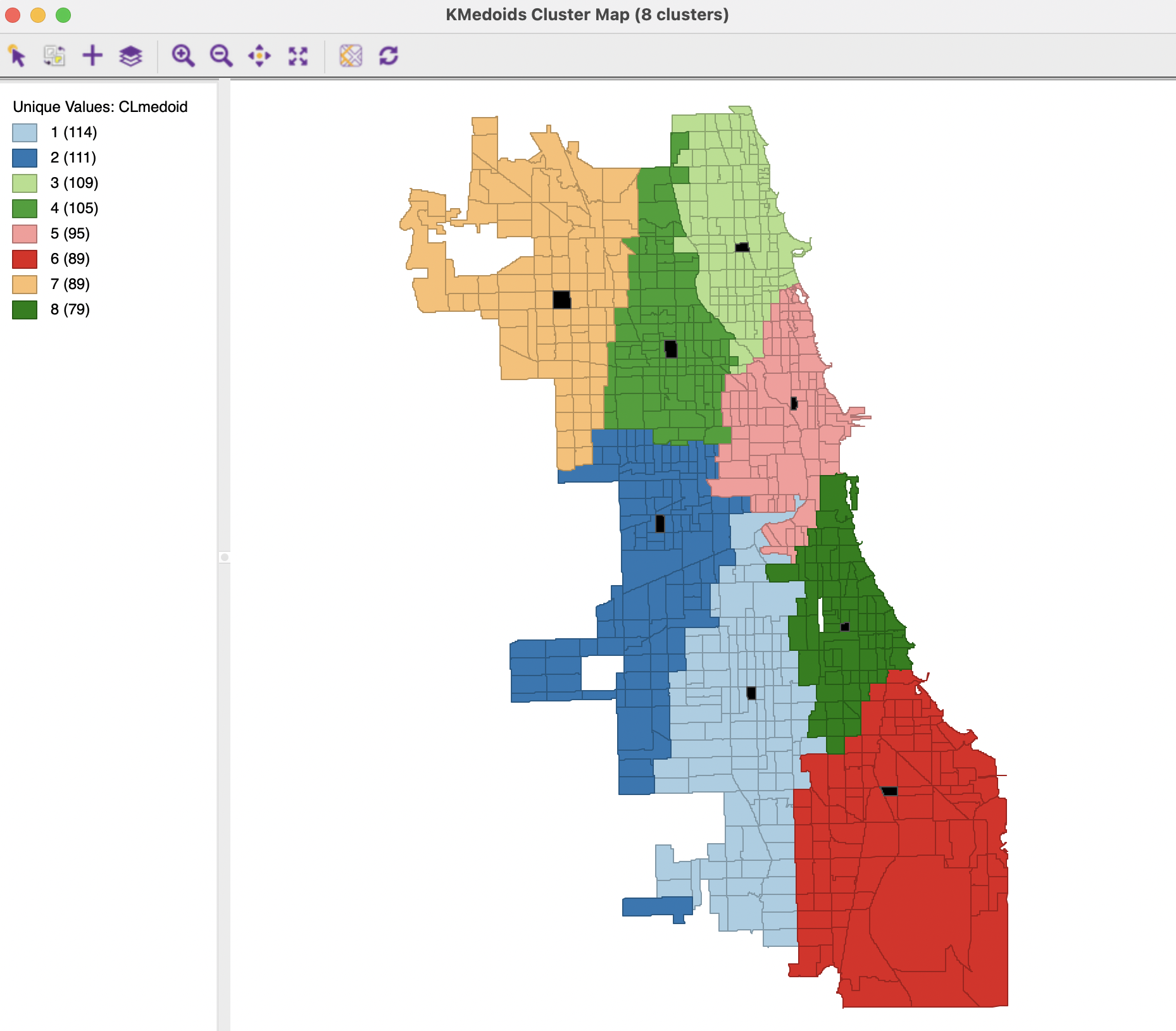
Figure 7.14: K-Medoids Cluster Map, k=8

7.3.4 Options and Sensitivity Analysis

The main option for K-Medoids is the choice of the Method. In addition to the default FastPAM, the algorithms FastCLARA and FastCLARANS are available as well. The latter two are large data methods. They will always perform (much) worse than FastPAM in small to medium-sized data sets.

In addition, there is a choice of Initialization Method between LAB and BUILD. In most circumstances, LAB is the preferred option, but BUILD is included for the sake of completeness and to allow for a full range of comparisons.

Each of these options has its own set of parameters.

7.3.4.1 CLARA parameters

The two main parameters that need to be specified for the CLARA method are the number of samples considered (by default set to 2) and the sample size. In addition, there is an option to include the best previous medoids in the sample.

7.3.4.2 CLARANS parameters

For CLARANS, the two relevant parameters pertain to the number of iterations and the sample rate. The former corresponds to the numlocal parameter in Ng and Han (2002), i.e., the number of times a local optimum is computed (default = 2). The sample rate pertains to the maximum number of neighbors that will be randomly sampled in each iteration (maxneighbors in the paper). This is expressed as a fraction of \(k \times (n - k)\). The default is to use the value of 0.025 recommended by Schubert and Rousseeuw (2019), which would yield a maximum neighbors of 20 (0.025 x 791) for each iteration in the Chicago example. Unlike PAM and CLARA, there is no initialization option.

CLARANS is a large data method and is optimized for speed (especially with large \(n\) and large \(k\)). It should not be used in smaller samples, where the exhaustive search carried out by PAM can be computed in a reasonable time.

---

34. Strictly speaking, k-medoids minimizes the average distance to the representative center, but the sum is easier for computational reasons.↩︎

35. Location-allocation problems are typically solved by means of integer programming or specialized heuristics, see, e.g., Church and Murray (2009), Chapter 11.↩︎

36. Detailed descriptions are given in Kaufman and Rousseeuw (2005), Chapters 2 and 3, as well as in Hastie, Tibshirani, and Friedman (2009), pp. 515-520, and Han, Kamber, and Pei (2012), pp. 454-457.↩︎

37. Clearly, with a sample size of 100%, CLARA becomes the same as PAM.↩︎

38. More precisely, the first sample consists of 40 + 2k random points. From the second sample on, the best k medoids found in a previous iteration are included, so that there are 40 + k additional random points. Also, in Schubert and Rousseeuw (2019), they suggested to use 80 + 4k and 10 repetitions for larger data sets. In the implementation in GeoDa, the latter is used for data sets larger than 100.↩︎

39. Schubert and Rousseeuw (2019) also consider 2.5% in larger data sets with 4 iterations instead of 2.↩︎

40. The map was created by first saving the selected cluster centers to a separate shape file and then using theGeoDa`’s multilayer functionality to superimpose the centers on the cluster map.↩︎