9.3 Including Geographical Coordinates in the Feature Set

Classic clustering procedures only deal with attribute similarity. They therefore do not guarantee that the resulting clusters are spatially contiguous, nor are they designed to do so. A number of ad hoc procedures have been suggested that start with the original result and proceed to create groupings where all members of the cluster become contiguous. In general, such approaches are unsatisfactory and none scale well to larger data sets. However, they are useful to illustrate the trade-offs involved in going from a non-spatial to a spatial solution.

Early approaches started with the solution of a standard clustering algorithm, and subsequently adjusted this in order to obtain contiguous regions, as in Openshaw (1973) and Openshaw and Rao (1995). For example, one could make every subset of contiguous observations a separate cluster, which would satisfy the spatial constraint. However, this would also increase the number of clusters. As a result, the initial value of \(k\) would no longer be valid. One could also manually move observations to an adjoining cluster and visually obtain contiguity while maintaining the same \(k\). However, this quickly becomes impractical when the number of observations is larger. A simple and scalable heuristic that implements this idea is illustrated in Section 9.5.

An alternative approach is to include the geometric centroids of the areal units as part of the clustering process by adding them as variables in the collection of attributes. Early applications of this idea can be found in Webster and Burrough (1972) and Murray and Shyy (2000), among others. However, while this tends to yield more geographically compact clusters, it does not guarantee contiguity. In other words, it introduces a soft spatial constraint.

In this context, it is again important to ensure that the coordinates are in projected units. Even though it is sometimes suggested in the literature to include latitude and longitude as additional features, this is incorrect. Only for projected units are the associated Euclidean distances meaningful.

Also, as pointed out earlier, the transformation of the variables, which is standard in the cluster procedures, may distort the geographical features when the East-West and North-South dimensions are very different. Due to the standardization, smaller distances in the shorter dimension will have the same weight as larger distances in the longer dimension, since the latter are more compressed in the standardization.

Unlike what was the case when clustering solely on geographic coordinates, keeping all the variables (including the non-geographical attributes) in a Raw format is not advisable. Due to the standardization, the result will be somewhat biased in favor of compactness in the longer dimension.

9.3.1 Implementation

To illustrate the inclusion of coordinates among the features, a K-Means analysis is carried out for the five urban dimension indices and the GDP per capita for the 184 municipalities in Ceará.

To set the baseline without coordinates, the six variables mobility, environ, housing, sanitation, infra and gdpcap are specified in the KMeans Clustering Settings dialog. All the default parameter values are used, with the number of clusters set to 12. The corresponding cluster map is shown in the left-hand panel of Figure 9.3, with the cluster characteristics listed in Figure 9.4.

The resulting spatial pattern is quite disparate, with cluster sizes ranging from 31 to 4. The only spatially compact cluster is the smallest, C12, consisting of 4 municipalities concentrated around the largest city of Fortaleza. In contrast, C11, also consisting of 4 municipalities, is made up of 4 completely spatially separated entities. For the other clusters, the ratio of subclusters to total cluster members, an indicator of fragmentation (higher values indicating more fragmentation), ranges from 0.38 for C3 (9 subclusters for 24 members) to 0.70 for C8 (7 subclusters for 10 members) and 0.71 for C5 and C6 (12 subclusters for 17 members). On the other hand, the overall separation is quite good, with a BSS/TSS ratio of 0.682.

As always, a careful interpretation of the cluster characteristics can be derived from the cluster center values for each of the variables, but this is beyond the current scope.

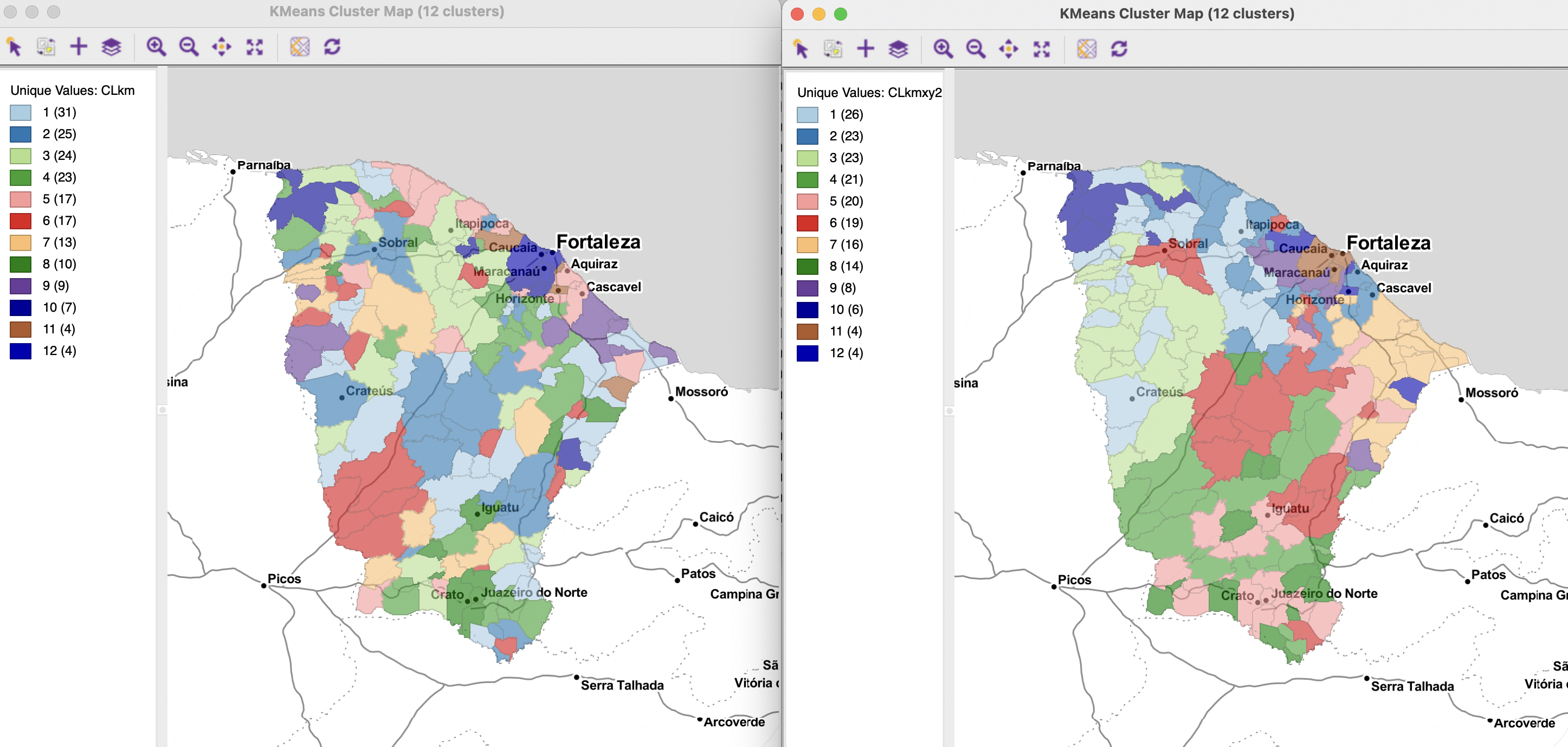
Figure 9.3: K-Means without and with X-Y Coordinates included

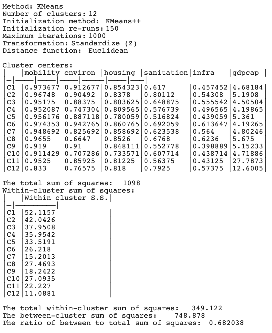
Figure 9.4: K-Means Cluster Characteristics

The coordinates are included among the features by adding <X-Centroids> and <Y-Centroids> to the six variables already specified in the KMeans Clustering Settings dialog. The rest of the interface remains unchanged.

The resulting cluster map is included as the right-hand panel in Figure 9.3, with the cluster characteristics in Figure 9.5. The clusters are more spatially compact, although by no means contiguous. C8 still consists of 9 subclusters (out of 14 members), and C1 and C2 consist of 8 (respectively, out of 26 and 23 cluster members). On the other hand, C10 only has two subclusters, and C3, C4, C7 and C9 only have 3. The BSS/TSS ratio decreases to 0.618, but it is not directly comparable, since it also includes the X and Y coordinates in the computations.

Since the X and Y coordinates were included in the analysis as regular variables, they are also included in the statistics for cluster centers in Figure 9.5.

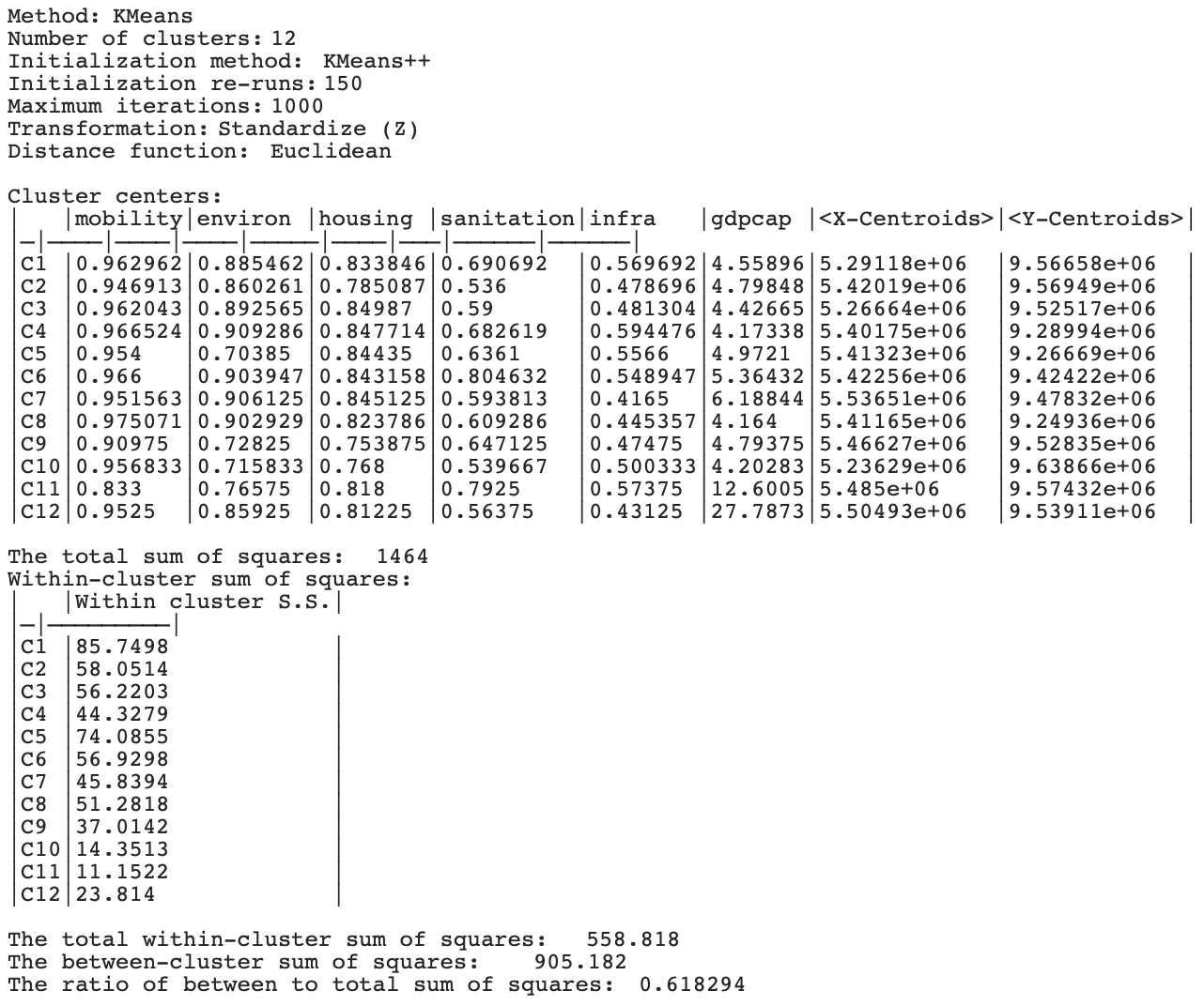
Figure 9.5: K-Means Cluster Characteristics with X-Y Coordinates

The results illustrate that including the coordinates may provide a form of spatial forcing, albeit imperfect. The outcome will tend to vary by clustering technique and the number of clusters specified (\(k\)), as well as by the number of attribute variables. In essence, this method gives equal weight to all the variables, so the higher the attribute dimension of the input variables, the less weight the spatial coordinates will receive. As a consequence, less spatial forcing will be possible with more variables. The heuristic outlined in the next section addresses this issue.