10.4 REDCAP
Whereas SCHC involves an agglomerative hierarchical approach and SKATER takes a divisive perspective, the REDCAP collection of methods suggested by Guo (2008) combines the two ideas (see also Guo and Wang 2011). In this approach, a distinction is made between the linkage update function (originally, single, complete and average linkage), and between the treatment of contiguity.
As Guo (2008) points out, the MST that is at the basis of the SKATER algorithm only takes into account first order contiguity among pairs of observations. Unlike the approach taken for SCHC, the contiguity relations are not updated to consider the newly formed clusters. As a result of this, observations that are part of a cluster that borders on a given spatial unit are not considered to be neighbors of that unit unless they are also first order contiguous. The distinction between a fixed contiguity relation and an updated spatial weights matrix is called FirstOrder and FullOrder. As a result, there are six possible methods, combining the three linkage functions with the two views of contiguity. In later work, Ward’s linkage was implemented as well.
In the discussion of density-based clustering in Chapter 20 of Volume 1, it was shown how the single-linkage dendrogram corresponds with a minimum spanning tree (MST). As a result, REDCAP’s FirstOrder-SingleLinkage and SKATER are identical. Since the FirstOrder methods are generally inferior to the FullOrder approaches, the latter are the main focus here.51
A careful consideration of the various REDCAP algorithms reveals that they essentially consist of three steps. First, a dendrogram for contiguity constrained hierarchical clustering is constructed, using the given linkage function. This yields the exact same dendrogram as produced by SCHC. Next, this dendrogram is turned into a spanning tree, using standard graph manipulation principles. Finally, the optimal cuts in the spanning tree are obtained using the same logic (and computations) as in SKATER, up to the desired level of \(k\).
10.4.1 Illustration - FullOrder-CompleteLinkage
To illustrate the REDCAP FullOrder-CompleteLinkage option for the Arizona county data, the results from SCHC (Section 10.2.1.1) and the logic from SKATER (Section 10.3.1) can be reused.
The first stage in the REDCAP algorithm consists of constructing a spanning tree that corresponds to a spatially constrained complete linkage hierarchical clustering dendrogram. For FullOrder, the steps to follow are the same as for complete linkage SCHC, yielding the dendrogram in Figure 10.7.
To create a spanning tree representation of this dendrogram, observations are connected following the merger of entities in the dendrogram. In the example, this means the first edge is between 8 and 14. In the second step, node 9 is connected to the cluster 8-14, but since 9 is only contiguous to 14, the edge becomes 9-14. The full sequence of edges is given in the list below. Whenever a new entity is connected to an existing cluster, it is connected to the only contiguous unit, or to the contiguous unit that is closest (using the distance measures in Figure 10.5 ):
- Step 1: 8-14
- Step 2: 9-14
- Step 3: 2-13
- Step 4: 4-12
- Step 5: 3-4
- Step 6: 11-8
- Step 7: 6-2
- Step 8: 5-4
- Step 9: 2-5
- Step 10: 7-11
- Step 11: 1-10
- Step 12: 11-12
- Step 13: 10-5
The resulting spanning tree is shown in Figure 10.22, with the sequence of steps marked in blue. The tree is largely the same as the MST in Figure 10.12, except that the edge between 11 and 2 is replaced by an edge between 5 and 2.
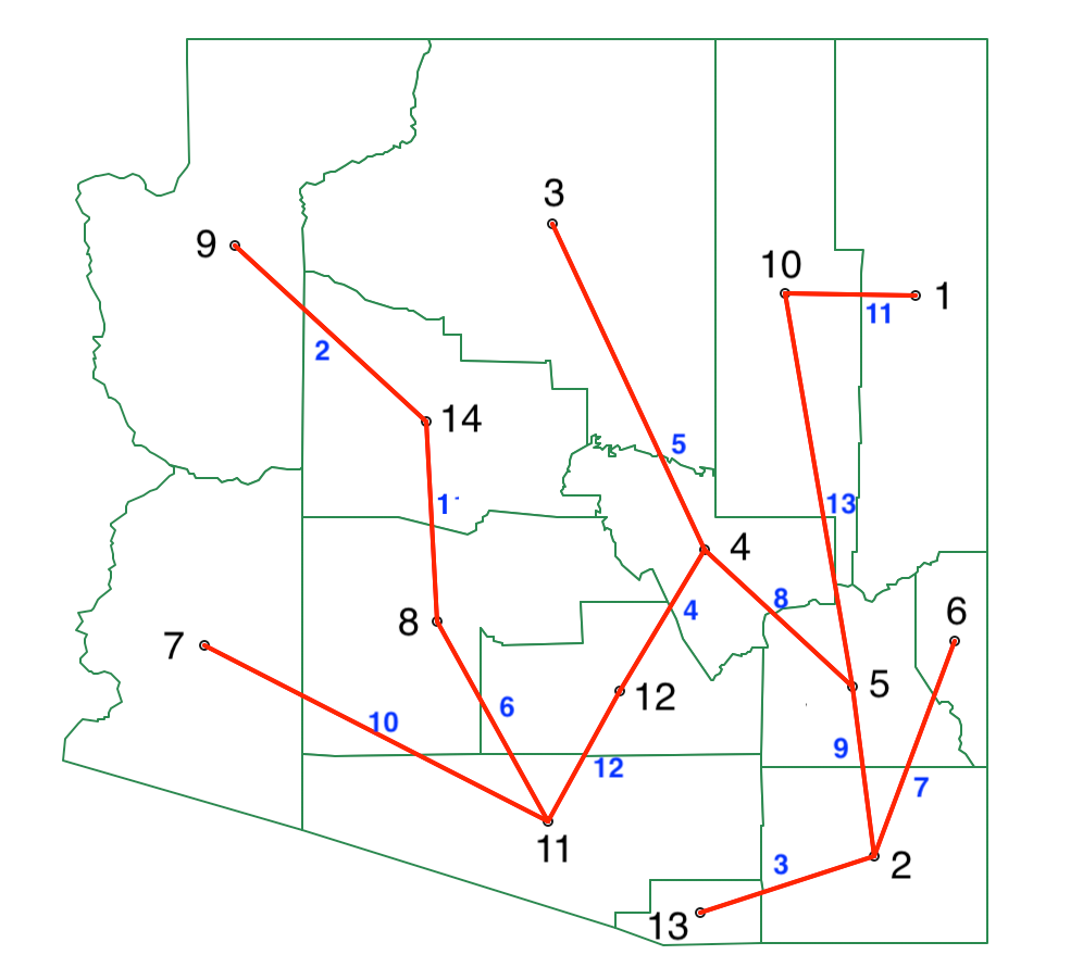
Figure 10.22: REDCAP FullOrder-CompleteLinkage spanning tree
At this point, an optimal cut in the minimum spanning tree is obtained using the same approach as for SKATER. Given the similarity of the two trees, a lot of the previous results can be reused. Only those subtrees affected by the new edge 5-2 replacing the edge 11-2 need to be considered again. Specifically, in the first step, these are the edges 5-2, 5-4, 4-12 and 11-12. The other results can be borrowed from the first step in SKATER, listed in Figure 10.13. The new results are given in Figure 10.23. As in the SKATER case, the first cut turns out to be between 5 and 10.
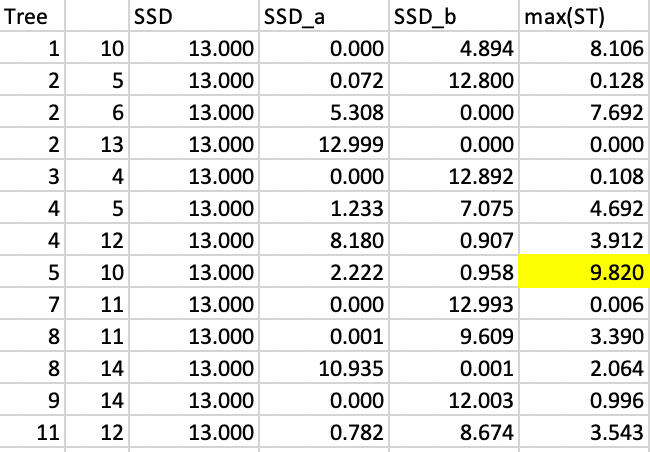
Figure 10.23: REDCAP step 1
The remaining steps also turn out to be the same as for the SKATER example, yielding the same layout for the four clusters as in Figure 10.16.
10.4.2 Implementation
The REDCAP algorithm is invoked from the drop down list associated with the cluster toolbar icon, as the last item in the subset highlighted in Figure 10.1. It can also be selected from the menu as Clusters > redcap.
Selecting this option brings up the REDCAP Settings dialog, which has the same structure as for SKATER, except that multiple methods are available. The panel provides a way to select the variables, the number of clusters and different options to determine the clusters. As for the previous methods, there is a Weights drop down list, where the contiguity weights must be specified. The REDCAP algorithms do not work without a spatial weights file.
Again, as for SKATER, it is possible to impose minimum bounds and to save the minimum spanning tree. These options are not further considered here (see Sections 10.3.2.1 and 10.3.2.2).
With the same six variables as before, the default method of FullOrder-WardLinkage (Ward’s linkage with dynamically updated spatial weights) yields the cluster map shown in Figure 10.24 for \(k\)=12.
Compared to the cluster map for SKATER in Figure 10.18, there are some broad similarities, although the layout is different in a number of important respects. The most striking difference is that the largest cluster is quite a bit smaller than before (77 observations vs 107). Also, there are now several sub-clusters in what was the dominant cluster for SKATER. However, there are still three singletons (compared to four) and all but four clusters consist of five or fewer observations.
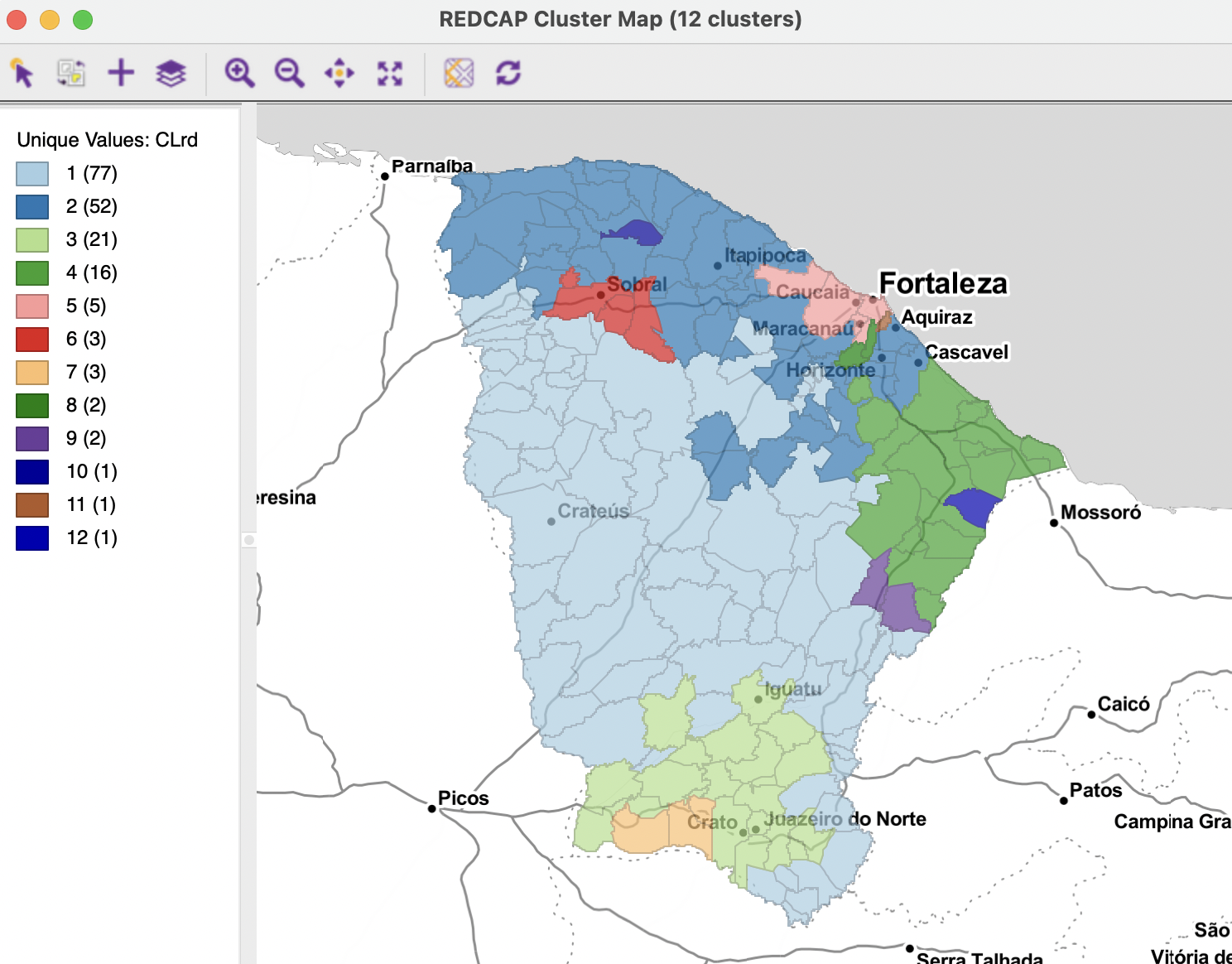
Figure 10.24: Ceará, REDCAP cluster map, k=12
The cluster characteristics are listed in Figure 10.25. The overall BSS/TSS ratio of 0.4627 is slightly better than SKATER (0.4325), an about the same (but slightly worse) than SCHC (0.4641).
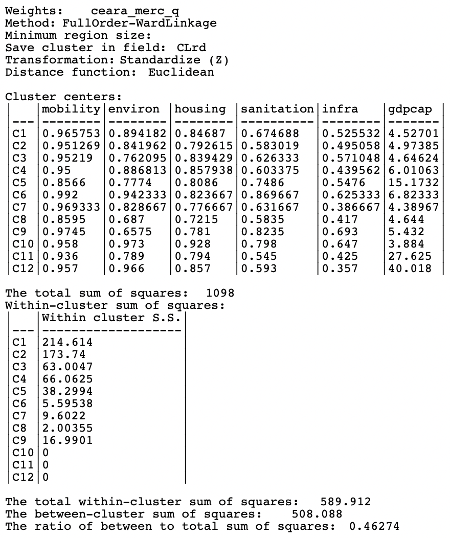
Figure 10.25: Ceará, REDCAP cluster characteristics, k=12
For comparison to SKATER,
GeoDaincludes FirstOrder-SingleLinkage as well, but the other FirstOrder methods are not implemented.↩︎