2.3 Principal Components
Principal components analysis has an eminent historical pedigree, going back to pioneering work in the early twentieth century by the statistician Karl Pearson (Pearson 1901) and the economist Harold Hotelling (Hotelling 1933). The technique is also known as the Karhunen-Loève transform in probability theory, and as empirical orthogonal functions or EOF in meteorology (see, for example, in applications of space-time statistics in Cressie and Wikle 2011; Wikle, Zammit-Mangion, and Cressie 2019).
The derivation of principal components can be approached from a number of different perspectives, all leading to the same solution. Perhaps the most common treatment considers the components as the solution of a problem of finding new variables that are constructed as a linear combination of the original variables, such that they maximize the explained variance. In a sense, the principal components can be interpreted as the best linear approximation to the multivariate point cloud of the data.
The point of departure is to organize \(n\) observations on \(k\) variables \(x_h\), with \(h = 1, \dots, k\), as a \(n \times k\) matrix \(X\) (each variable is a column in the matrix). In practice, each of the variables is typically standardized, such that its mean is zero and variance equals one. This avoids problems with (large) scale differences between the variables (i.e., some are very small numbers and others very large). For such standardized variables, the \(k \times k\) cross product matrix \(X'X\) corresponds to the correlation matrix (without standardization, this would be the variance-covariance matrix).2
The goal is to find a small number of new variables, the so-called principal components, that explain the bulk of the variance (or, in practice, the correlation) in the original variables. If this can be accomplished with a much smaller number of variables than in the original set, the objective of dimension reduction will have been achieved.
Each principal component \(z_u\) is a linear combination of the original variables \(x_h\), with \(h\) going from \(1\) to \(k\) such that: \[z_u = a_1 x_1 + a_2 x_2 + \dots + a_k x_k\] The mathematical problem is to find the coefficients \(a_h\) such that the new variables maximize the explained variance of the original variables. In addition, to avoid an indeterminate solution, the coefficients are scaled such that the sum of their squares equals \(1\).
A full mathematical treatment of the derivation of the optimal solution to this problem is beyond the current scope (for details, see, e.g., Lee and Verleysen 2007, chap. 2). Nevertheless, obtaining a basic intuition for the mathematical principles involved is useful.
The coefficients by which the original variables need to be multiplied to obtain each principal component can be shown to correspond to the elements of the eigenvectors of \(X'X\), with the associated eigenvalue giving the explained variance. Even though the original data matrix \(X\) is typically not square (of dimension \(n \times k\)), the cross-product matrix \(X'X\) is of dimension \(k \times k\), so it is square and symmetric. As a result, all the eigenvalues are real numbers, which avoids having to deal with complex numbers.
Operationally, the principal component coefficients are obtained by means of a matrix decomposition. One option is to compute the spectral decomposition of the \(k \times k\) matrix \(X'X\), i.e., of the correlation matrix. As shown in Section 2.2.2.1, this yields: \[X'X = VGV',\] where \(V\) is a \(k \times k\) matrix with the eigenvectors as columns (the coefficients needed to construct the principal components), and \(G\) a \(k \times k\) diagonal matrix of the associated eigenvalues (the explained variance).
A principal component for each observation is obtained by multiplying the row of standardized observations by the column of eigenvalues, i.e., a column of the matrix \(V\). More formally, all the principal components are obtained concisely as: \[XV.\]
A second, and computationally preferred way to approach this is as a singular value decomposition (SVD) of the \(n \times k\) matrix \(X\), i.e., the matrix of (standardized) observations. From Section 2.2.2.2, this follows as \[X = UDV',\] where again \(V\) (the transpose of the \(k \times k\) matrix \(V'\)) is the matrix with the eigenvectors of \(X'X\) as columns, and \(D\) is a \(k \times k\) diagonal matrix, containing the square root of the eigenvalues of \(X'X\) on the diagonal.3 Note that the number of eigenvalues used in the spectral decomposition and in SVD is the same, and equals \(k\), the column dimension of \(X\).
Since \(V'V = I\), the following result obtains when both sides of the SVD decomposition are post-multiplied by \(V\): \[XV = UDV'V = UD.\] In other words, the principal components \(XV\) can also be obtained as the product of the orthonormal matrix \(U\) with a diagonal matrix containing the square root of the eigenvalues, \(D\). This result is important in the context of multidimensional scaling, considered in Chapter 3.
It turns out that the SVD approach is the solution to viewing the principal components explicitly as a dimension reduction problem, originally considered by Karl Pearson. The observed vector on the \(k\) variables \(x\) can be expressed as a function of a number of unknown latent variables \(z\), such that there is a linear relationship between them: \[ x = Az, \] where \(x\) is a \(k \times 1\) vector of the observed variables, and \(z\) is a \(p \times 1\) vector of the (unobserved) latent variables, ideally with \(p\) much smaller than \(k\). The matrix \(A\) is of dimension \(k \times p\) and contains the coefficients of the transformation. Again, in order to avoid indeterminate solutions, the coefficients are scaled such that \(A'A = I\), which ensures that the sum of squares of the coefficients associated with a given component equals one.
Instead of maximizing explained variance, the objective is now to find \(A\) and \(z\) such that the so-called reconstruction error is minimized.4
Importantly, different computational approaches to obtain the eigenvalues and eigenvectors (there is no analytical solution) may yield opposite signs for the elements of the eigenvectors. However, the eigenvalues will be the same. The sign of the eigenvectors will affect the sign of the resulting component, i.e., positives become negatives. For example, this can be the difference between results based on a spectral decomposition versus SVD.
In a principal component analysis, the interest typically focuses on three main results. First, the principal component scores are used as a replacement for the original variables. This is particularly relevant when a small number of components explain a substantial share of the original variance. Second, the relative contribution of each of the original variables to each principal component is of interest. Finally, the variance proportion explained by each component in and of itself is also important.
2.3.1 Implementation
Principal components are invoked from the drop down list created by the toolbar Clusters icon (Figure 2.1) as the top item (more precisely, the first item in the dimension reduction category). Alternatively, from the main menu, Clusters > PCA gets the process started.
The illustration uses ten variables that characterize the efficiency of community banks, based on the observations for 2013 from the Italy Community Bank sample data set (see Algeri et al. 2022):
- CAPRAT: ratio of capital over risk weighted assets
- Z: z score of return on assets (ROA) + leverage over the standard deviation of ROA
- LIQASS: ratio of liquid assets over total assets
- NPL: ratio of non-performing loans over total loans
- LLP: ratio of loan loss provision over customer loans
- INTR: ratio of interest expense over total funds
- DEPO: ratio of total deposits over total assets
- EQLN: ratio of total equity over customer loans
- SERV: ratio of net interest income over total operating revenues
- EXPE: ratio of operating expenses over total assets
Some descriptive statistics are listed in Figure 2.3. An analysis of individual box plots (not shown) reveals that most distributions are quite skewed, with only NPL, INTR and DEPO not showing any outliers. SERV is the only variable with outliers at the low end of the distribution. All the other variables have a considerable number of outlying observations at the high end (see Algeri et al. 2022 for a substantive discussion of the variables).
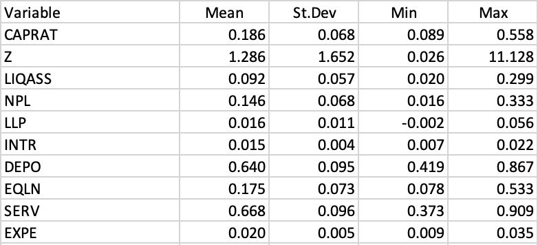
Figure 2.3: Italy Bank Characteristics Descriptive Statistics
The correlation matrix (not shown) includes both very strong linear relations between pairs of variables as well as very low ones. For example, NPL is highly correlated with SERV (-0.90) and LLP (0.64), as is CAPRATA with EQLN (0.87), but LIQASS is essentially uncorrelated with NPL (-0.004) and SERV (0.01).
Selection of PCA brings up the PCA Settings Menu, which is the main interface to specify all the settings. This interface has a similar structure for all multivariate analyses and is shown in Figure 2.4.
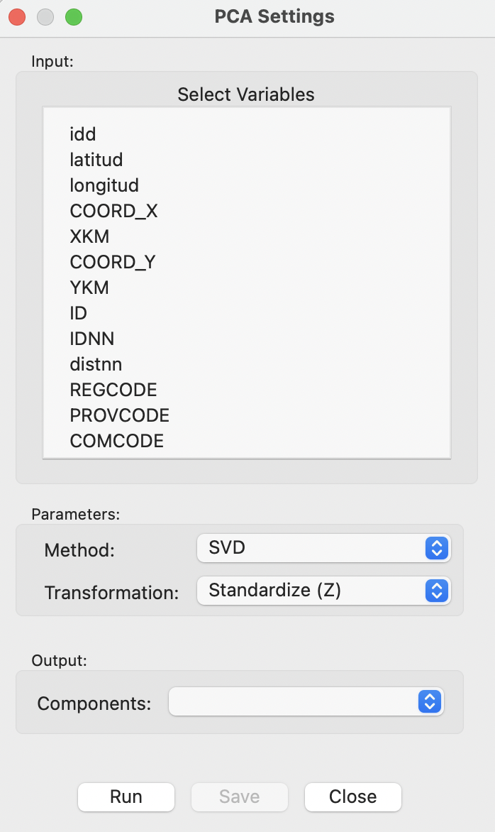
Figure 2.4: PCA Settings Menu
The top dialog is the interface to Select Variables. The default Method to compute the various coefficients is SVD. The other option is Eigen, which uses spectral decomposition. By default, all variables are used as Standardize (Z), such that the mean is zero and the standard deviation is one.5
The Run button computes the principal components and brings up the results in the right-hand panel, as shown in Figure 2.5.
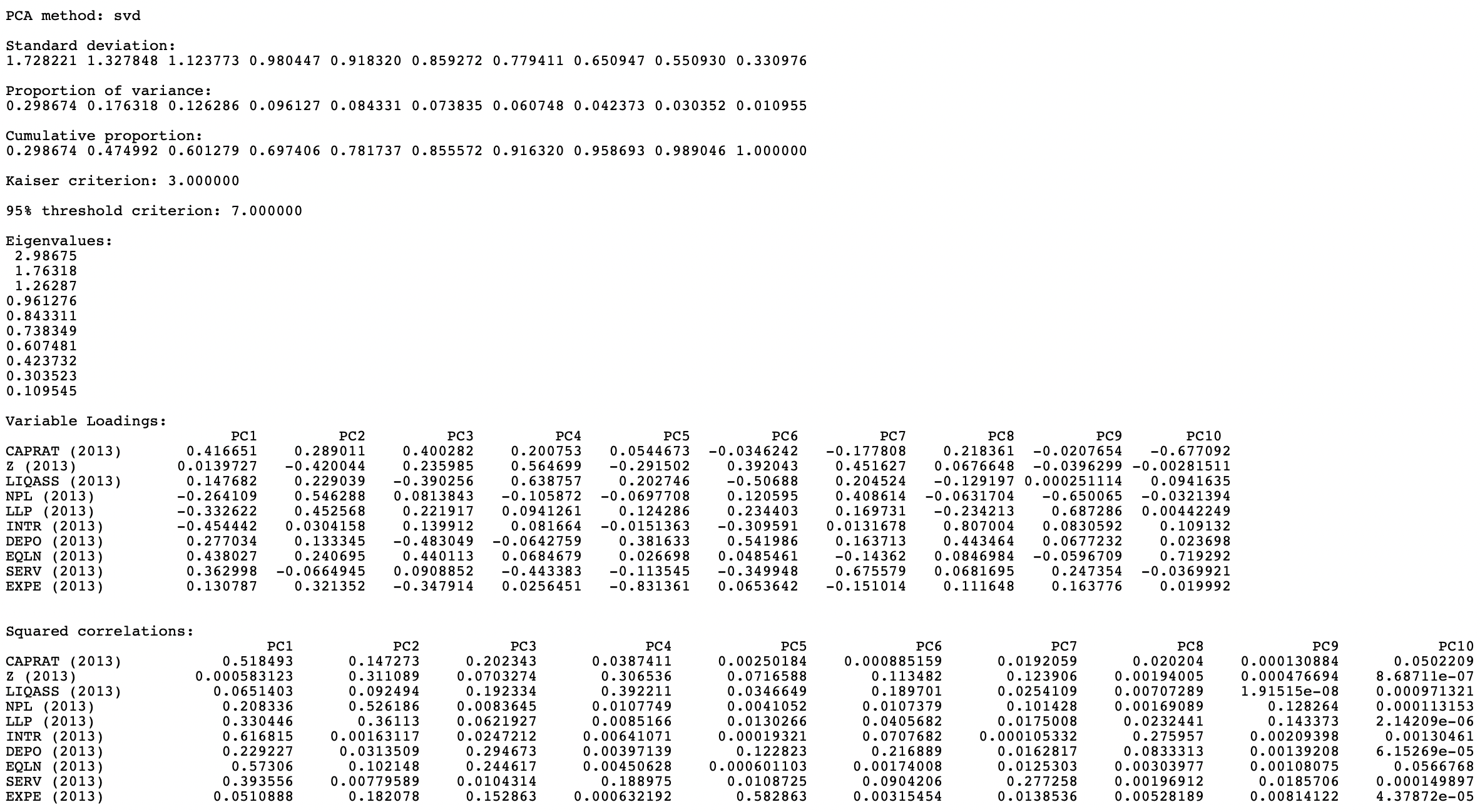
Figure 2.5: PCA Results
The result summary is evaluated in more detail in Section 2.3.2.
2.3.1.1 Saving the principal components
Once the computation is finished, the resulting principal components become available to be added to the Data Table as new variables. The Components drop-down list suggests the number of components based on the 95% variance criterion (see Section 2.3.2). In the example, this is 7.
Invoking the Save button brings up a dialog to specify the variable names for the principal components, with as default PC1, PC2, etc. These variables are added to the Data Table and become available for any subsequent analysis or visualization. This is illustrated in Figure 2.6 for seven components based on the ten original bank variables.
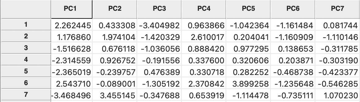
Figure 2.6: Principal Components in the Data Table
2.3.2 Interpretation
The panel with summary results (Figure 2.5) provides several statistics pertaining to the variance decomposition, the eigenvalues, the variable loadings and the contribution of each of the original variables to the respective components.
2.3.2.1 Explained variance
After listing the PCA method (here the default SVD), the first item in the results panel gives the Standard deviation explained by each of the components. It corresponds to the square root of the Eigenvalues (each eigenvalue equals the variance explained by the corresponding principal component), which are listed as well. In the example, the first eigenvalue is 2.98675, which is thus the variance of the first component. Consequently, the standard deviation is the square root of this value, i.e., 1.728221, given as the first item in the list.
The sum of all the eigenvalues is 10, which equals the number of variables, or, more precisely, the rank of the matrix \(X'X\). Therefore, the proportion of variance explained by the first component is 2.98675/10 = 0.2987, as reported in the list. Similarly, the proportion explained by the second component is 0.1763, so that the cumulative proportion of the first and second component amounts to 0.2987 + 0.1763 = 0.4750. In other words, the first two components explain a little less than half of the total variance.
The fraction of the total variance explained is listed both as a separate Proportion and as a Cumulative proportion. The latter is typically used to choose a cut-off for the number of components. A common convention is to take a threshold of 95%, which would suggest 7 components in the example.
An alternative criterion to select the number of components is the so-called Kaiser criterion (Kaiser 1960), which suggests to take the components for which the eigenvalue exceeds 1. In the example, this would yield 3 components (they explain slightly more than 60% of the total variance).
The bottom part of the results panel is occupied by two tables that have the original variables as rows and the components as columns.
2.3.2.2 Variable loadings
The first table that relates principal components to the original variables shows the Variable Loadings. For each principal component (column), this lists the elements of the corresponding eigenvector. The eigenvectors are standardized such that the sum of the squared coefficients equals one. The elements of the eigenvector are the coefficients by which the (standardized) original variables need to be multiplied to construct each component (see Section 2.3.2.3).
It is important to keep in mind that the signs of the loadings may switch, depending on the algorithm that is used in the computation. However, the absolute value of the coefficients remains the same. In the example, setting Method to Eigen yields the loadings shown in Figure 2.7.
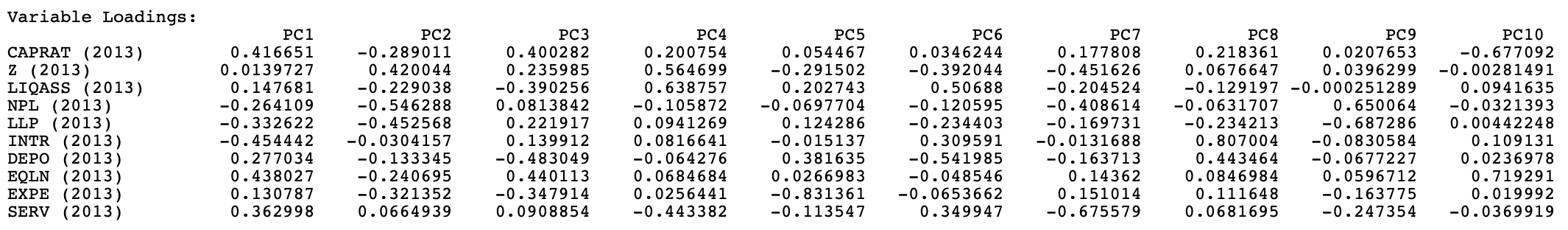
Figure 2.7: Variable Loadings Using the EIGEN Mehtod
For PC2, PC6, PC7, and PC9, the signs for the loadings are the opposite of those reported in Figure 2.5. This needs to be kept in mind when interpreting the actual value (and sign) of the components and when using the components as variables in subsequent analyses (e.g., regression) and visualization (see Section 2.4).
When the original variables are all standardized, each eigenvector coefficient gives a measure of the relative contribution of a variable to the component in question.
2.3.2.3 Variable loadings and principal components
The detailed computation of the principal components is illustrated for the first two observations on the first component in Figure 2.8. The names of the standardized variables are listed in the left-most column, followed by the principal component loadings (the values in the PC1 column in Figure 2.5). The next column shows the standardized values for each variable for the first observation. These are multiplied by the loading in column four, with the sum listed at the bottom. The value of 2.2624 matches the entry in the first row under PC1 in Figure 2.6.
Similarly, the value of 1.1769 for the second row under PC1 is obtained at the bottom of column 6. Similar calculations can be carried out to verify the other entries.
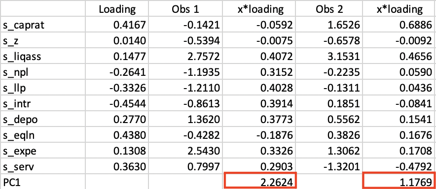
Figure 2.8: Principal Component Calculation
2.3.2.4 Substantive interpretation - squared correlation
The interpretation and substantive meaning of the principal components can be a challenge. In factor analysis, a number of rotations are applied to clarify the contribution of each variable to the different components. The latter are then imbued with meaning such as “social deprivation”, “religious climate”, etc. Principal component analysis tends to stay away from this, but nevertheless, it is useful to consider the relative contribution of each variable to the respective components.
The table labeled as Squared correlations lists those statistics between each of the original variables in a row and the principal component listed in the column. Each row of the table shows how much of the variance in the original variable is explained by each of the components. As a result, the values in each row sum to one.
More insightful is the analysis of each column, which indicates which variables are important in the computation of the matching component. In the example, INTR (61.7%), EQLN (57.3%) and CAPRAT (51.8%) dominate the contributions to the first principal component. In the second component, the main contributor is NPL (52.6%), as well as Z (31.1%). This provides a way to interpret how the multiple dimensions along the ten original variables are summarized into the main principal components.
Since the correlations are squared, they do not depend on the sign of the eigenvector elements, unlike the loadings.
The standardization should not be done mechanically, since there are instances where the variance differences between the variables are actually meaningful, e.g., when the scales on which they are measured have a strong substantive meaning (e.g., in psychology).↩︎
Since the eigenvalues equal the variance explained by the corresponding component, the diagonal elements of \(D\) are thus the standard deviation explained by the component.↩︎
The concept of reconstruction error is somewhat technical. If \(A\) were a square matrix, one could solve for \(z\) as \(z = A^{-1}x\), where \(A^{-1}\) is the inverse of the matrix \(A\). However, due to the dimension reduction, \(A\) is not square, so something called a pseudo-inverse or Moore-Penrose inverse must be used. This is the \(p \times k\) matrix \((A'A)^{-1}A'\), such that \(z = (A'A)^{-1}A'x\). Furthermore, because \(A'A = I\), this simplifies to \(z = A'x\) (of course, so far the elements of \(A\) are unknown). Since \(x = Az\), if \(A\) were known, \(x\) could be found as \(Az\), or, as \(AA'x\). The reconstruction error is then the squared difference between \(x\) and \(AA'x\). The objective is to find the coefficients for \(A\) that minimize this expression. For an extensive technical discussion, see Lee and Verleysen (2007), Chapter 2.↩︎
A full list of the standardization options in
GeoDais given in Chapter 2 of Volume 1.↩︎