11.2 Automatic Zoning Procedure (AZP)
The automatic zoning procedure (AZP) was initially suggested by Openshaw (1977) as a way to address some of the consequences of the modifiable areal unit problem (MAUP). In essence, it consists of a heuristic to find the best set of combinations of contiguous spatial units into \(p\) regions, minimizing the within sum of squares as a criterion of homogeneity. The number of regions needs to be specified beforehand, as in all the other clustering methods considered so far.
The problem is NP-hard, so that it is impossible to find an analytical solution. Also, in all but toy problems, a full enumeration of all possible layouts is impractical. In Openshaw and Rao (1995), the original slow hill-climbing heuristic is augmented with a number of other approaches, such as tabu search and simulated annealing, to avoid the problem of becoming trapped in a local solution. None of the heuristics guarantee that a global solution will be found, so sensitivity analysis and some experimentation with different starting points is very important.
Addressing the sensitivity of the solution to starting points is the motivation behind the automatic regionalization with initial seed location (ARiSeL) procedure, proposed by Duque and Church in 2004.52
It is important to keep in mind that just running AZP with the default settings is not sufficient. Several parameters need to be manipulated to get a good sense of what the best (or, a better) solution might be. This may seem a bit disconcerting at first, but it is intrinsic to the use of a heuristic that does not guarantee global optimality.
11.2.1 AZP Heuristic
The original AZP heuristic is a local optimization procedure that cycles through a series of possible swaps between spatial units at the boundary of a given region. The process starts with an initial feasible solution, i.e., a grouping of \(n\) spatial units into \(p\) regions that consist of contiguous units. The initial solution can be constructed in a number of different ways, but it is critical that it satisfies the contiguity constraint.
For example, a solution can be obtained by growing a set of contiguous regions from \(p\) randomly selected seed units by adding neighboring locations until the contiguity constraint can no longer be met. In addition, the order in which neighbors are assigned to growing regions can be based on how close they are in attribute space. Alternatively, to save on having to compute the associated WSS, the order can be random. This process yields an initial list of regions and an allocation of each spatial unit to one and only one of the regions.
To initiate the search for a local optimum, a random region from the list is selected and its set of neighboring spatial units considered for a swap, one at a time. More specifically, the impact on the objective function is assessed of a move of that unit from its original region to the region under consideration. Such a move is only allowed if it does not break the contiguity constraint in the origin region. If it improves on the overall objective function, i.e., the total within sum of squares, then the move is carried out.
With a new unit added to the region under consideration, its neighbor structure (spatial weights) needs to be updated to include new neighbors from the spatial unit that was moved and that were not part of the original neighbor list.
The evaluation is continued and moves implemented until the (updated) neighbor list is exhausted.
At this point, the process moves to the next randomly picked region from the region list and repeats the evaluation of all the neighbors. When the region list is empty (i.e., all initial regions have been evaluated), the whole operation is repeated with the updated region list until the improvement in the objective function falls below a critical convergence criterion.
The heuristic is local in that it does not try to find the globally best move. It considers only one neighbor of one region at a time, without checking on the potential swaps for the other neighbors or regions. As a result, the process can easily get trapped in a local optimum.
11.2.1.1 Illustration
The logic behind the AZP heuristic is illustrated for the Arizona county example, with \(p\) = 4.
The point of departure is a random initial feasible solution with four clusters, for example as depicted in Figure 11.2. The clusters are labeled a (7-9-14), b (1-3-10), c (4-8-11-12), and d (2-5-6-13). Since each cluster consists of contiguous units, it is a feasible solution.
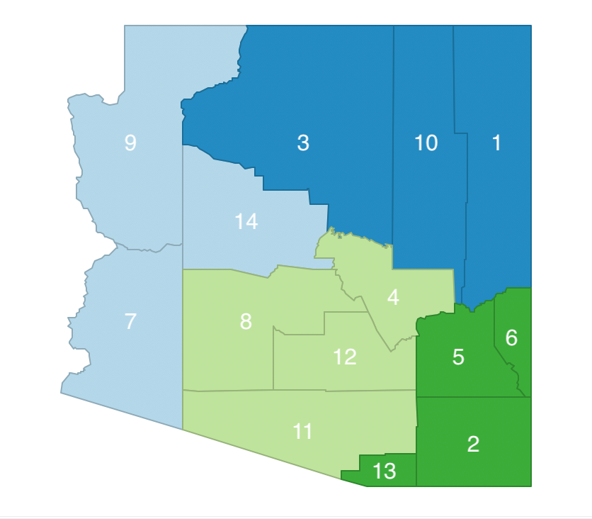
Figure 11.2: Arizona AZP initial feasible solution
The associated within sum of squares for each cluster is computed in Figure 11.3. The values in the column SUE are used to compute the cluster average (\(\bar{x}_p\)), the squared values are listed in column SUE^2. For each cluster, the within SSD is calculated as \(\sum_i x_i^2 - n_p \bar{x}_p^2\). For example, for cluster a, this yields \(1.7760 - 3 \times (-0.602)^2 = 0.6905\) (rounded). The Total Within SSD corresponding to this allocation is 6.2408, listed at the bottom of the figure.
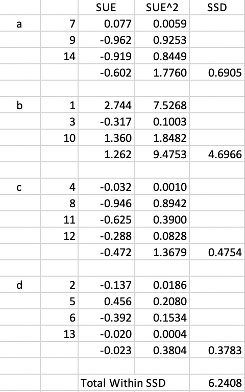
Figure 11.3: Arizona AZP initial Total Within SSD
Following the AZP logic, a list of zones is constructed as Z = [a, b, c, d]. In addition, each observation is allocated to a zone, contained in a list, as W = [b, d, b, c, d, d, a, c, a, b, c, c, d, a].
Next, one of the zones is picked randomly, e.g., zone c, shown with its labels removed in Figure 11.4. It is then removed from the list, with is updated as Z = [a, b, d]. After evaluating the neighbor list for zone c, this process is repeated for another element of the list, until the list is empty.
Associated with cluster c is a list of its neighbors. These are identified in Figure 11.4 as C = [2, 3, 5, 7, 10, 13, 14].
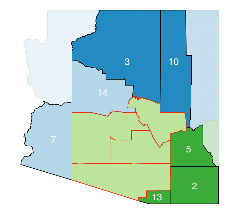
Figure 11.4: Arizona AZP initial neighbor list
The next step consists of randomly selecting one of the elements of the neighbor list, e.g., 2, and to evaluate its move from its current cluster (b) to cluster c, highlighted by changing its color in the map. However, as shown in Figure 11.5, in this case, swapping observation 2 between b and c would break the contiguity in cluster b (13 would become an isolate), so this move is not allowed. As a result, 2 stays in cluster b for now.
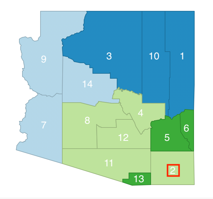
Figure 11.5: Arizona AZP step 1 neighbor selection - 2
Since the previous move was not accepted, a new move is attempted by randomly selecting another element from the remaining neighbor list C = [3, 4, 5, 7, 10, 13, 14]. For example, observation 14 could be considered for a move from cluster a to cluster c, as shown in Figure 11.6. This move does not break the contiguity between the remaining elements in cluster a (7 remains a neighbor of 9), so it is potentially allowed.
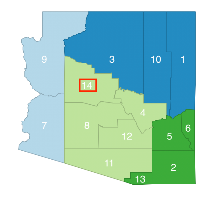
Figure 11.6: Arizona AZP step 2 neighbor selection - 14
This potential swap would result in cluster a consisting of 2 elements and cluster c of 5. The corresponding updated sums of squared deviations are given in Figure 11.7. The Total Within SSD becomes 6.2492, which is not an improvement over the current objective function (6.2408). As a consequence, this swap is rejected and observation 14 stays in cluster a.
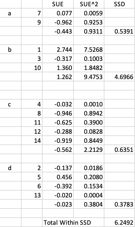
Figure 11.7: Arizona AZP step 2 Total Within SSD
At this point, observation 14 has been removed from the neighbor list, which becomes C = [3, 4, 5, 7, 10, 13]. A new neighbor is randomly selected, e.g., observation 3. The swap involves a move from cluster b to cluster c, as in Figure 11.8. This move does not break the contiguity of the remaining elements in cluster b (10 and 1 remain neighbors), so it is potentially allowed.
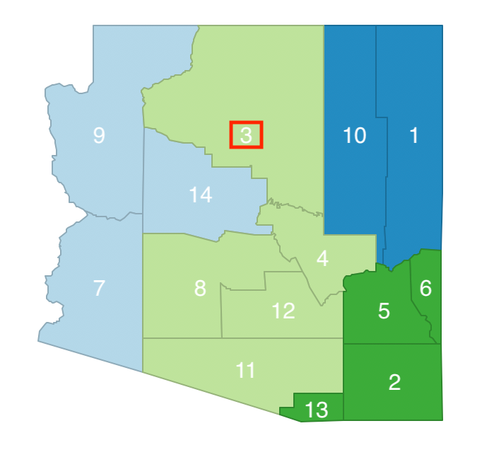
Figure 11.8: Arizona AZP step 3 neighbor selection - 3
Cluster b now consists of 2 elements and cluster c has 5. The associated SSD and Total Within SSD are listed in Figure 11.9. The swap of 3 from b to c yields an improvement in the overall objective from 6.2408 to 2.5213, so it is implemented.
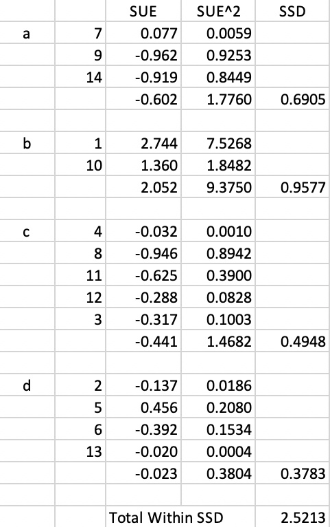
Figure 11.9: Arizona AZP step 3 Total Within SSD
The next step is to re-evaluate the list of neighbors of the updated cluster c. It turns out that observation 9 must be included as an additional neighbor to the list. The neighbor list thus becomes C = [4, 5, 7, 10, 13, 9].
The process continues by evaluating potential neighbor swaps until the list C is empty. At that point, the original list Z = [a, b, d] is reconsidered and another unit is randomly selected. Its neighbor set is identified and the procedure is repeated until list Z is empty.
After the first full iteration, the whole process is repeated, starting with an updated list Z = [a, b, c, d]. This is carried out until convergence, i.e., until the improvement in the overall objective becomes less than a pre-specified threshold.
11.2.2 Tabu Search
The major idea behind methods to avoid being trapped in a local minimum amounts is to allow non-improving moves at one or more stages in the optimization process. This purposeful moving in the wrong direction provides a way to escape from potentially inferior local optima.
A tabu search is one such method. It was originally suggested in the context of mixed integer programming by Glover (1977), but has found wide applicability in a range of combinatorial problems, including AZP (originally introduced in this context by Openshaw and Rao 1995).
One aspect of the local search in AZP is that there may be a lot of cycling, in the sense that spatial units are moved from one region to another and at a later step moved back to the original region. In order to avoid this, a tabu search maintains a so-called tabu list that contains a number of (return) steps that are prohibited.
With a given regional layout, all possible swaps are considered from a list of candidates
from the adjoining neighbors. Each of these neighbors that is not in the current tabu list is considered
for a possible swap, and the best swap is selected. If the best swap improves the overall objective
function (the total within sum of squares), then it is implemented. This is the standard approach. In addition,
the reverse move (moving the neighbor back to its original region) is added to the
tabu list. In practice, this means that this entity cannot be returning to its original cluster for \(R\) iterations, where \(R\) is the length
of the tabu list, or the Tabu Length parameter in GeoDa.
If the best swap does not improve the overall objective, then the next available tabu move is considered, a so-called aspirational move. If the latter improves on the overall objective, it is carried out. Again, the reverse move is added to the tabu list. However, if the aspirational move does not improve the objective, then the original best swap is implemented anyway and again its reverse move is also added to the tabu list. In a sense, rather than making no move, a move is made that makes the overall objective (slightly) worse. The number of such non-improving moves is limited by the ConvTabu parameter.
The tabu approach can dramatically improve the quality of the end result of the search. However, a critical parameter is the length of the tabu list, or, equivalently, the number of iterations that a tabu move cannot be considered. The results can be highly sensitive to the selection of this parameter, so that some experimentation is recommended (for examples, see the detailed experiments in Duque, Anselin, and Rey 2012).
In all other respects, the tabu search AZP uses the same steps as outlined for the original AZP heuristic.
11.2.3 Simulated Annealing
Another method to avoid local minima is so-called simulated annealing. This approach originated in physics, and is also known as the Metropolis algorithm, commonly used in Markov Chain Monte Carlo simulation (Metropolis et al. 1953). The idea is to introduce some randomness into the decision to accept a non-improving move, but to make such moves less and less likely as the heuristic proceeds.
If a move (i.e., a move of a spatial unit into a new region) does not improve the objective function, it can still be accepted with a probability based on the so-called Boltzmann equation. It compares the (negative) exponential of the relative change in the objective function to a 0-1 uniform random number. The exponent is divided by a factor, called the temperature, which is decreased (lowered) as the process goes on.
Formally, with \(\Delta O/O\) as the relative change in the objective function and \(r\) as a draw from a
uniform 0-1 random distribution, the condition of acceptance of a non-improving move \(v\) is:
\[ r < e^\frac{-\Delta O/O}{T(v)},\]
where \(T(v)\) is the temperature at annealing step \(v\).53
Typically \(v\) is constrained so that only a limited number of such annealing moves are allowed per iteration. In
addition, only a limited number of iterations are allowed (in GeoDa, this is controlled by the maxit parameter).
The starting temperature is typically taken as \(T = 1\) and gradually reduced at each annealing step \(v\)
by means of a cooling rate \(c\), such that:
\[T(v) = c.T(v-1).\]
In GeoDa, the default cooling rate is set to 0.85, but typically some experimentation may be
needed. Historically, Openshaw and Rao (1995) suggested values for the cooling rate for AZP between 0.8 and 0.95.
The effect of the cooling rate is that \(T(v)\) becomes smaller, so that the value in the negative exponent term \(a = \frac{-\Delta O/O}{T(v)}\) becomes larger. Since the relevant expression is \(e^{-a}\), the larger \(a\) is, the smaller will be the negative exponential. The resulting value is compared to a uniform random number \(r\), with mean 0.5. Therefore, smaller and smaller values on the right-hand side of the Boltzmann equation will result in less and less likely acceptance of non-improving moves.
In AZP, the simulated annealing approach is applied to the evaluation step of the neighboring units, i.e., whether or not the move of a spatial unit from its origin region to the region under consideration will improve the objective.
As for the tabu search, the simulated annealing logic only pertains to selecting a neighbor swap. Otherwise, the heuristic is not affected.
11.2.4 ARiSeL
The ARiSeL approach, which stands for automatic regionalization with initial seed location, is an alternative way to select the initial feasible solution. In the original AZP formulation, this initial solution is based on a random choice of \(p\) seeds, and the initial feasible regions are grown around these seeds by adding the nearest neighbors. It turns out that the result of AZP is highly sensitive to this starting point.
Duque and Church proposed the ARiSeL alternative, based on seeds obtained from a Kmeans++ procedure (see Section 6.2.3). This yields better starting points for growing a whole collection of initial feasible regions. Then the best such solution is chosen as the basis for a tabu search or other search procedure.
11.2.5 Using the Outcome from Another Cluster Routine as the Initial Feasible Region
Rather than using a heuristic to construct a set of initial feasible regions, the outcome of another spatially constrained clustering algorithm could be used. This is particularly appropriate for hierarchical methods like SCHC, SKATER and REDCAP, where observations cannot be moved once they are assigned to a (sub-)branch of the minimum spanning tree.
GeoDa allows the allocation that resulted from other methods (like spatially constrained hierarchical methods) to be used as the starting point for AZP. This is an alternative to the random generation of a starting point.
An alternative perspective on this approach is to view it as a way to improve the results of the hierarchical methods, where, as mentioned, observations can become trapped in a branch of the dendrogram. The flexible swapping inherent to AZP allows for the search for potential improvements at the margin. In practice, this particular application of AZP has almost always resulted in a better solution, where observations at the edge of previous regions are swapped to improve the objective function.
11.2.6 Implementation
The AZP algorithm is invoked from the drop down list associated with the cluster toolbar icon, as the first item in the subset highlighted in Figure 11.1. It can also be selected from the menu as Clusters > AZP.
The AZP Settings interface takes the familiar form, the same as for the other spatially constrained cluster methods. In addition to the variables and the spatial weights, the number of clusters needs to be specified, and the method of interest selected: AZP (the default local search), AZP-Tabu Search, or AZP-Simulated Annealing. As before, there is also an option to set a minimum bound.
Two important choices are the search method and the initialization. The latter includes the option to specify a feasible initial region and side-step the customary random initialization. These options are discussed in turn. The other options are the same as before and are not further considered.
The same six variables are used as in the previous chapters, and the number of regions is set to 12 in order to obtain comparable results.
11.2.7 Search Options
The search options are selected from the Method drop down list. Each has its own set of parameters.
To facilitate comparison, recall that the BSS/TSS ratio for K-Means was 0.682, 0.4641 for SCHC, 0.4325 for SKATER, and 0.4627 for REDCAP.
11.2.7.1 Local Search
The default option is the local search, invoked as AZP. It does not have any special parameter settings. The initialization options are kept to the default.
The resulting cluster map and characteristics are given in Figure 11.10. The clusters are better balanced in size than for the hierarchical solutions and there only one singleton. However, there remain six clusters with four or fewer observations. The spatial layout is somewhat different from the results obtained so far, although some broad patterns are similar.
The characteristics on the right indicate the method (AZP) and the Initial value of objective function as 751.889. This is the WSS, which is reduced to 689.208 in the Final value. The usual cluster centers are reported, as well as the cluster-specific WSS. The final BSS/TSS ratio is 0.3723, the worst result so far for the spatially constrained methods. As mentioned, the default settings almost never provide a satisfactory result for AZP, and some experimenting is necessary.
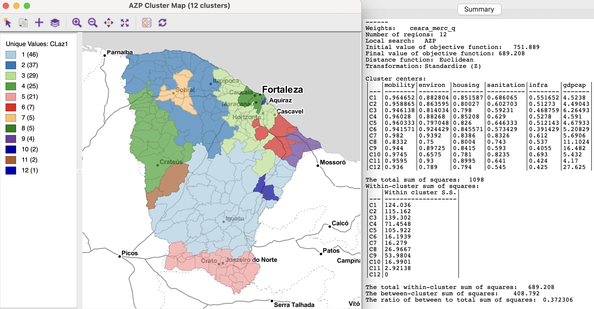
Figure 11.10: Ceará AZP clusters for p=12, local search
11.2.7.2 Tabu search
AZP-Tabu Search is the second item in the Method drop down list. The default parameters are for a Tabu Length (10) and for the ConvTabu, i.e., the number of non-improving moves allowed. Initially this is left blank, since it is computed internally, as the maximum of 10 and \(n / p\), which yields 15 in the example. With the default settings, the final value of the objective becomes 689.083 (the initial value is the same as before, since this is not affected by the search method), yielding a BSS/TSS ratio of 0.3724 (not shown).
Some experimenting can improve this to 0.4004 by using a Tabu length of 50 with 25 non-improving moves. This is better than the default AZP, but still worse than the hierarchical results. The cluster map and detailed cluster characteristics are shown in Figure 11.11. The final value of the WSS is 658.326. The spatial layout is again different, with one singletons and six clusters with five or fewer observations. However, closer examination reveal several commonalities with previous results.
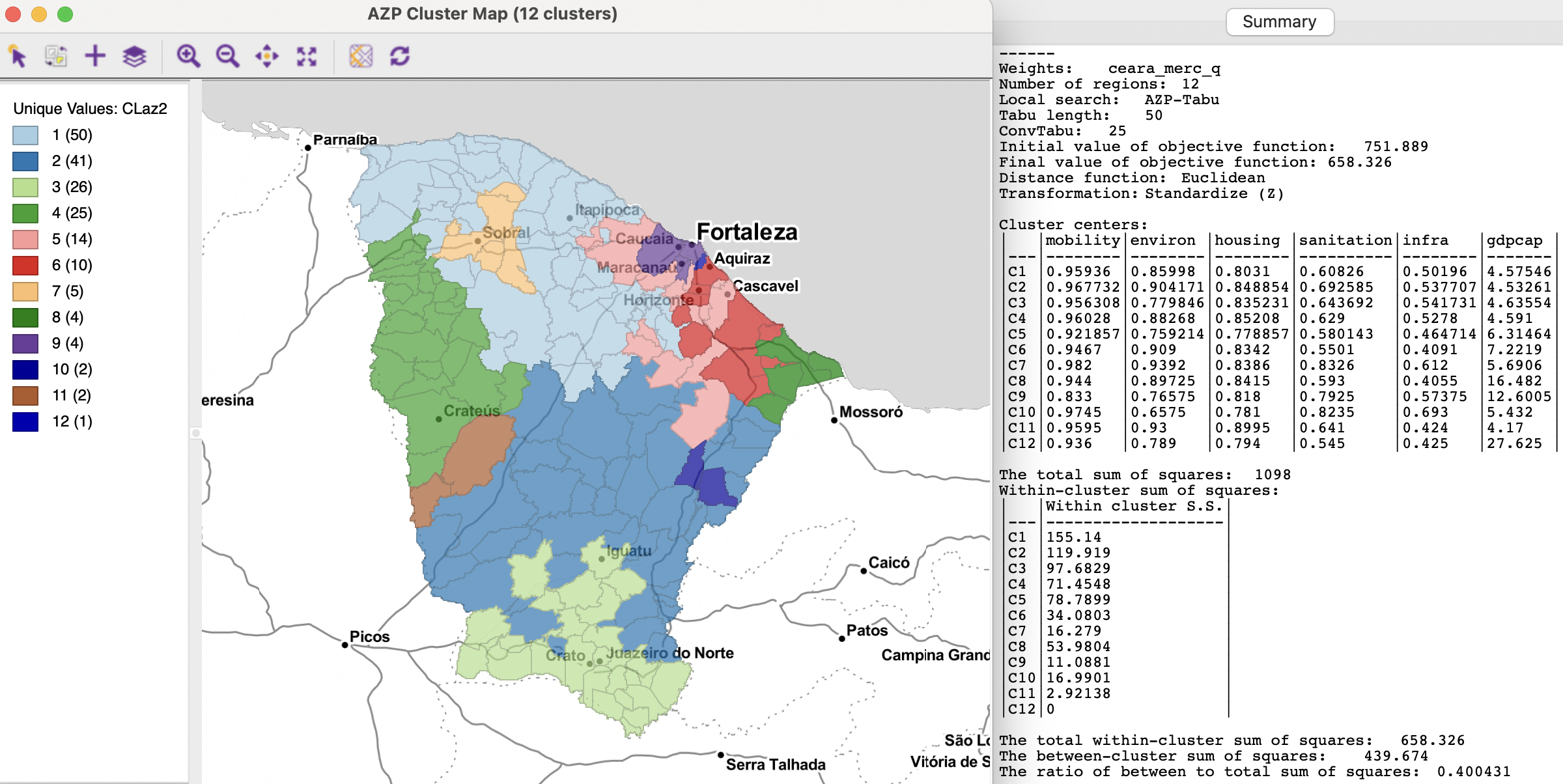
Figure 11.11: Ceará AZP clusters for p=12, tabu search
11.2.7.3 Simulated annealing
The third option in the Method drop down list is AZP-Simulated Annealing. This method is controlled by two important parameters: Cooling Rate and Maxit. The cooling rate is the rate at which the annealing temperature is allowed to decrease, with a default value of 0.85. Maxit sets the number of iterations allowed for each swap, with a default value of 1.
For these default settings, a final BSS/RSS ratio of 0.4146 is obtained, an improvement over the previous results (the final WSS is 642.753). However, the outcome of the simulated annealing approach is very sensitive to the two parameters. Some experimentation reveals a BSS/TSS ratio of 0.4225 for a cooling rate of 0.85 with maxit=5, and a ratio of 0.4368 for a cooling rate of 0.8 with maxit=5. The latter result is depicted in Figure 11.12. The final ratio is now in the same range as the results for the hierarchical methods.
The cluster map contains a singleton (in the higher GDP area focused around the city of Fortaleza), but only two other clusters have four or fewer observations. The overall result is much better balanced than before. However, there are also some strange connections due to common vertices obtained with the queen contiguity criterion. For example, Cluster 1 and Cluster 5 seem to cross to the east of Crateús, and there is a strange connection between Cluster 6 and Cluster 2 south of Horizonte. This illustrates the potential sensitivity of the results to peculiarities of the spatial weights.
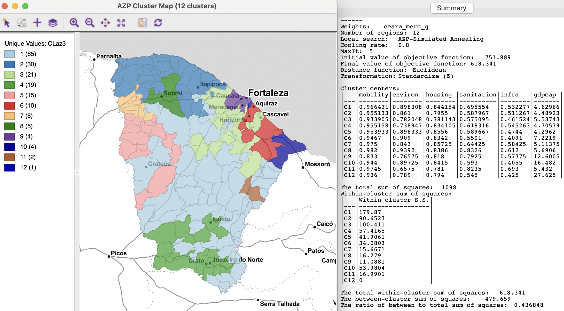
Figure 11.12: Ceará AZP clusters for p=12, simulated annealing search
11.2.8 Initialization Options
The AZP algorithm is very sensitive to the selection of the initial feasible solution. One easy approach is to assess whether a different random seed might yield a better solution. This is readily accomplished by means of the Use Specified Seed check box in the AZP Settings dialog.
Alternative is to use the Kmeans++ logic from ARiSeL and to specify the initial regions explicitly.
11.2.8.1 ARiSeL
The ARiSeL option is selected by means of a check box in the dialog. There is also the option to change the number of re-runs (the default is 10), which provides additional flexibility. With the default setting and using the best simulated annealing approach (cooling rate of 0.8 with maxit=5), this yields an improved solution with a BSS/TSS ratio of 0.4492. In addition, with the number of re-runs set to 50, the best AZP result so far is obtained (although still not quite as good as SCHC), depicted in Figure 11.13. This yields a BSS/TSS ratio of 0.4627. Note also how the Initial Value of the objective function, i.e., the total WSS of the initial feasible solution has improved to 687.865 from the previous 751.889. However, in spite of this better initial solution, the final result is not always better. This very much also depends on the other choices for the algorithm parameters.
The resulting layout shows several similarities with the cluster map in Figure 11.12, although now there are two singletons, and several more small clusters (with less than 10 observations).
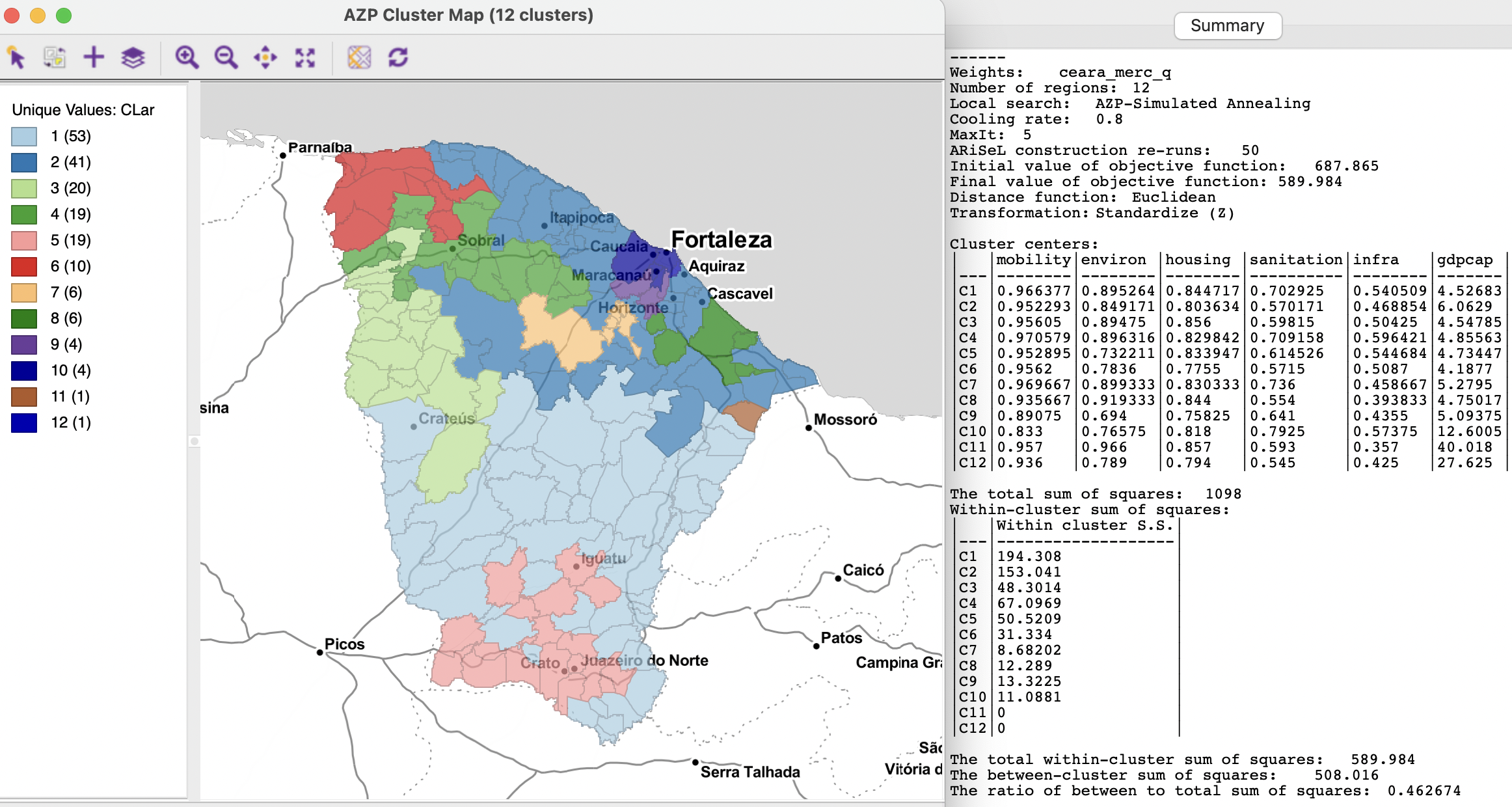
Figure 11.13: Ceará AZP clusters for p=12, simulated annealing search with ARiSeL
11.2.8.2 Initial regions
A final way to potentially improve on the solution is to take a previous spatially constrained cluster assignment as the initial feasible solution. This is accomplished by checking the Initial Regions box and selecting a suitable cluster indicator variable from the drop down list.
The approach is illustrated with the SCHC cluster assignment from Section 10.2.2 as the initial feasible solution. It is used in combination with an AZP simulated annealing algorithm with cooling rate 0.8 and maxit=5. The Initial Value of the objective function is now 588.391, i.e., the final value from the SCHC solution. This is even slightly better than the final value for the ARiSeL result (589.984), and by far the lowest initial value used up to this point.
The outcome is shown in Figure 11.14. The final BSS/TSS ratio improves to 0.5036, with a final objective value of 545.063, the best result so far. The cluster map has three singletons and is dominated by one large region. The layout is largely the same as for the SCHC solution, with some minor adjustments at the margin.
This illustrates the importance of fine tuning the various settings for the AZP algorithm, as well as the utility of leveraging several different algorithms.
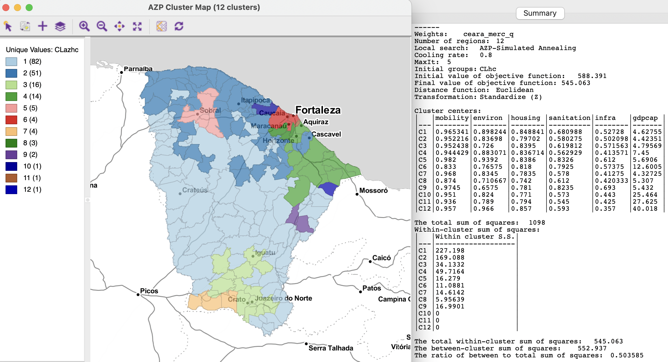
Figure 11.14: Ceará AZP clusters for p=12, simulated annealing search with SCHC initial regions
The origins of this method date back to a presentation at the North American Regional Science Conference in Seattle, WA, November 2004. See the description in the clusterpy documentation at http://www.rise.abetan16.webfactional.com/risem/clusterpy/clusterpy0_9_9/exogenous.html#arisel-description.↩︎
The typical application of simulated annealing is a maximization problem, in which the negative sign in the exponential of the Boltzmann equation is absent. However, since in the current case the problem is one of minimizing the total within sum or squares, the exponent becomes the negative of the relative change in the objective function.↩︎