10.3 SKATER
The SKATER algorithm introduced by Assunção et al. (2006), and later extended in Teixeira, Assunção, and Loschi (2015) and Aydin et al. (2018), is based on the optimal pruning of a minimum spanning tree that reflects the contiguity structure among the observations.47
As in SCHC, the point of departure is a dissimilarity matrix that only contains weights for contiguous observations. This matrix is represented as a graph with the observations as nodes and the contiguity relations as edges.
The full graph is reduced to a minimum spanning tree (MST), i.e., such that all nodes are connected (no isolates or islands) and there is exactly one path between any pair of nodes (no loops). As a result, the n nodes are connected by n-1 edges, such that the overall between-node dissimilarity is minimized. This yields a starting sum of squared deviations or SSD as \(\sum_i (x_i - \bar{x})^2\), where \(\bar{x}\) is the overall mean.
The objective is to reduce the overall SSD by maximizing the between SSD, or, alternatively, minimizing the sum of within SSD. The MST is pruned by selecting the edge whose removal increases the objective function (between group dissimilarity) the most. To accomplish this, each potential split is evaluated in terms of its contribution to the objective function.
More precisely, for each tree T, the difference between the overall objective value and the sum of the values for each subtree is evaluated: \(\mbox{SSD}_T - (\mbox{SSD}_a + \mbox{SSD}_b)\), where \(\mbox{SSD}_a, \mbox{SSD}_b\) are the contributions of each subtree. The contribution is computed by first calculating the average for that subtree and then obtaining the sum of squared deviations.48 The cut in the subtree is selected where the difference \(\mbox{SSD}_T - (\mbox{SSD}_a + \mbox{SSD}_b)\) is the largest.49
At this point, the process is repeated for the new set of subtrees to select an optimal cut. It continues until the desired number of clusters (\(k\)) has been reached.
Like SCHC, this is a hierarchical clustering method, but here the approach is divisive instead of agglomerative. In other words, it starts with a single cluster, and finds the optimal split into subclusters until the value of \(k\) is satisfied. Because of this hierarchical nature, once the tree is cut at one point, all subsequent cuts are limited to the resulting subtrees. In other words, once an observation ends up in a pruned branch of the tree, it cannot switch back to a previous branch. This is sometimes viewed as a limitation of the SKATER algorithm.
In addition, the contiguity constraint is based on the original configurations and does not take into account new neighbor relations that follow from the combination of different observations into clusters, as was the case for SCHC.
10.3.1 Pruning the Minimum Spanning Tree
TThe SKATER algorithm is again illustrated by means of the Arizona county example. The first step in the process is to reduce the information for contiguous pairs in the distance matrix of Figure 10.5 (highlighted in red) to a minimum spanning tree (MST). The result is shown in Figure 10.12, against the backdrop of the Arizona county map.
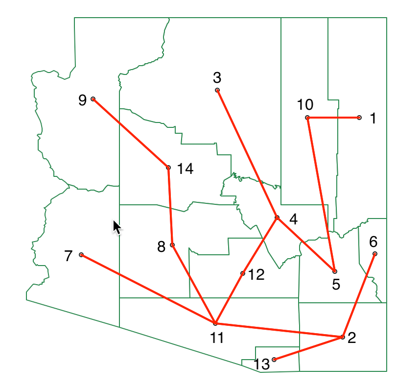
Figure 10.12: SKATER minimum spanning tree
At this point, every possible cut in the MST needs to be evaluated in terms of its contribution to reducing the overall sum of squared deviations (SSD). Since the unemployment rate variable is standardized, its mean is zero by construction. As a result, the total sum of squared deviations is the sum of squares. In the example, this sum is 13.50
The vertices for each possible cut are shown as the first two columns in Figure 10.13, with the node number given for the start and endpoint of the edge in the graph. For each subtree, the corresponding SSD must be calculated. The next step then implements the optimal cut such that the total SSD decreases the most, i.e., max[\(\mbox{SSD}_T - (\mbox{SSD}_a + \mbox{SSD}_b)\)], where \(\mbox{SSD}_T\) is the SSD for the corresponding tree, and \(\mbox{SSD}_a\) and \(\mbox{SSD}_b\) are the totals for the subtrees corresponding to the cut.
In order to accomplish this, the SSD for each subtree that would result from the cut is computed as \(\sum_i x_i^2 - n_k \bar{x}_k^2\), with \(\bar{x}_k\) as the mean for the average value for the subtree and \(n_k\) as the number of elements in the subtree.
For example, for the cut 1-10, the vertex 1 becomes a singleton, so its SSD is 0 (\(SSD_a\) in the fourth column and first row in Figure 10.13). For vertex 10, the subtree consists of all elements other than 1, with a mean of -0.211 and an SSD of 4.894 (\(SSD_b\) in the fifth column and first row in Figure 10.13). Consequently, the contribution to reducing the overall SSD amounts to 13.000 - (0 + 4.894) = 8.106.
In a similar fashion, the SSD for each possible subtree is calculated. This yields the results in Figure 10.13. The largest decrease in overall SSD is achieved by the cut between 5 and 10, which gives a reduction of 9.820.
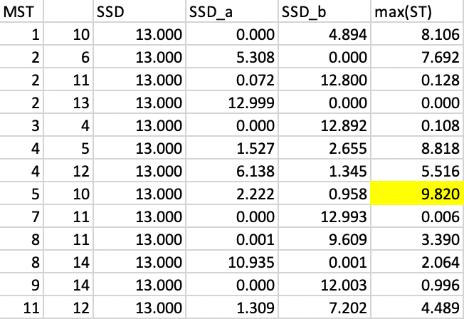
Figure 10.13: SKATER step 1
The updated MST after cutting the link between 5 and 10 is shown in Figure 10.14, yielding two initial subtrees.
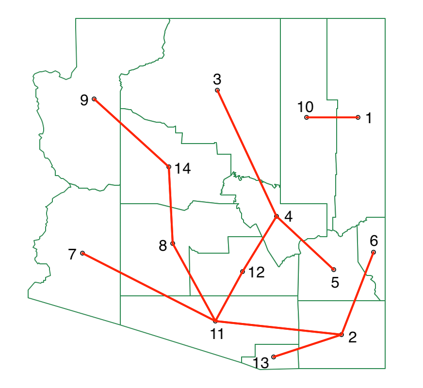
Figure 10.14: SKATER minimum spanning tree - first split
The process is now repeated, looking for the greatest decrease in overall SSD. The data is separated into two subtrees, one for 1-10 and the other for the remaining vertices. In each, the SSD for the subtree follows as 0.958 for 1-10 and 2.222 for the other cluster. For each possible cut, the SSD for the corresponding subtrees must be recalculated. The greatest contribution towards reducing the overall SSD is offered by a cut between 8 and 11, with a contribution of 1.441.
At this point, only one more cut is needed (since \(k\)=4). Neither subtree can match the contribution of 0.958 obtained by 1-10 (since the split yields two single observations, the decrease in SSD equals the total SSD for the subtree). Consequently, no further calculations are needed. The final MST shown in Figure 10.15.
Figure 10.15: SKATER minimum spanning tree - final split
The matching cluster map is given in Figure 10.16. It contains two singletons, a cluster of nine observations and one consisting of three.
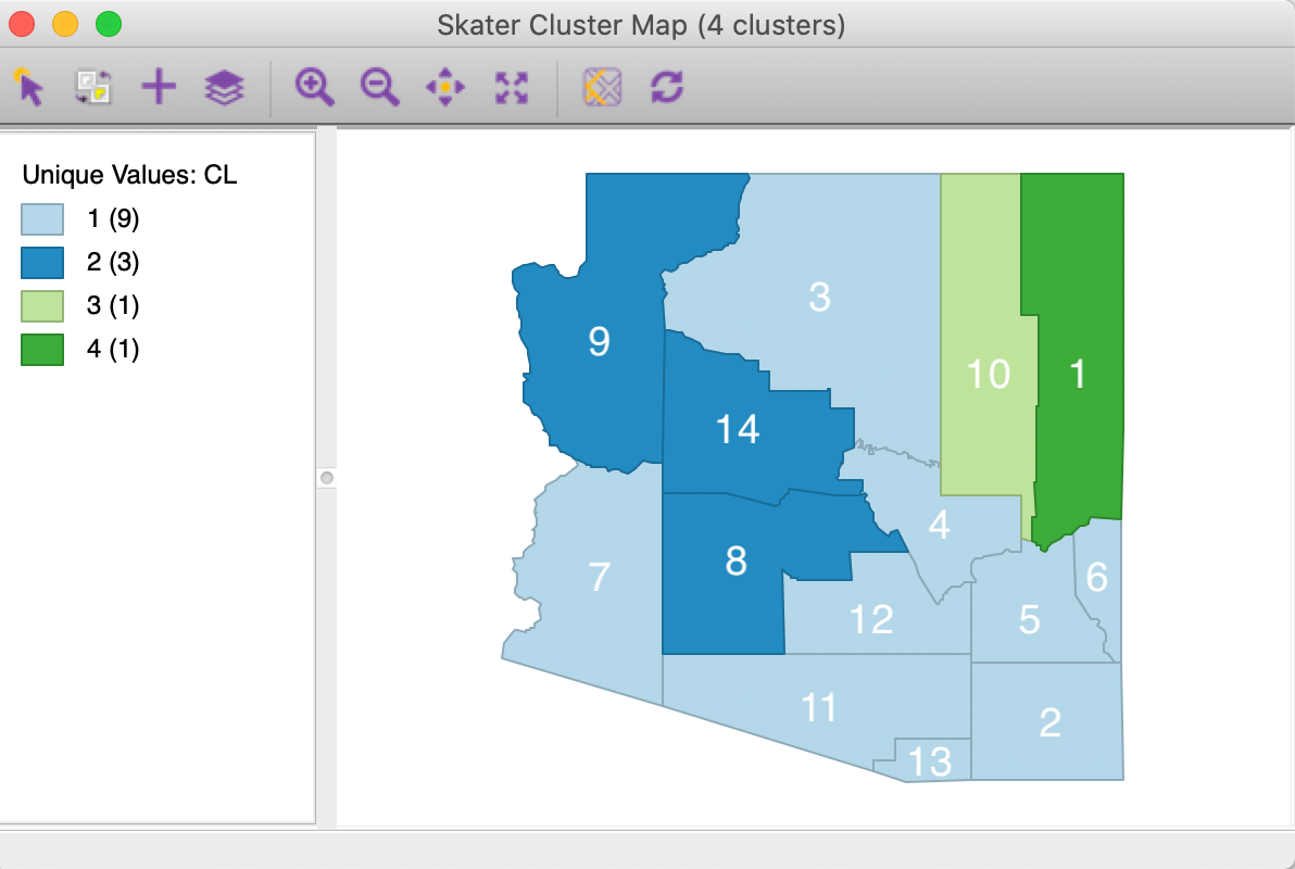
Figure 10.16: SKATER cluster map, k=4
10.3.2 Implementation
The SKATER algorithm is invoked from the drop down list associated with the cluster toolbar icon, as the second item in the subset highlighted in Figure 10.1. It can also be selected from the menu as Clusters > skater.
This brings up the Skater Settings dialog, which consists of the two customary main panels. As for SCHC, in addition to the variable selection, a spatial weights file must be specified (queen contiguity in the example). The same six variables are used as in the previous examples. The other options are the same as before, with two additional selections: saving the Spanning Tree (Section 10.3.2.1), and setting a Minimum Bound or Minimum Region Size (Section 10.3.2.2).
To illustrate the logic of SKATER, the first cut is highlighted in Figure 10.17, with the MST graph derived from queen contiguity super-imposed on the spatial areal units. The first step in the algorithm cuts the MST into two parts. This generates two sub-regions: one consisting of 177 observations, the other made up of seven municipalities. The green rectangle identifies the edge in the MST where the first cut is made.
The algorithm proceeds by creating subsets of the existing regions, either from the seven observations or from the 177 others. Each subset forms a self-contained sub-tree of the initial MST, corresponding to a region.
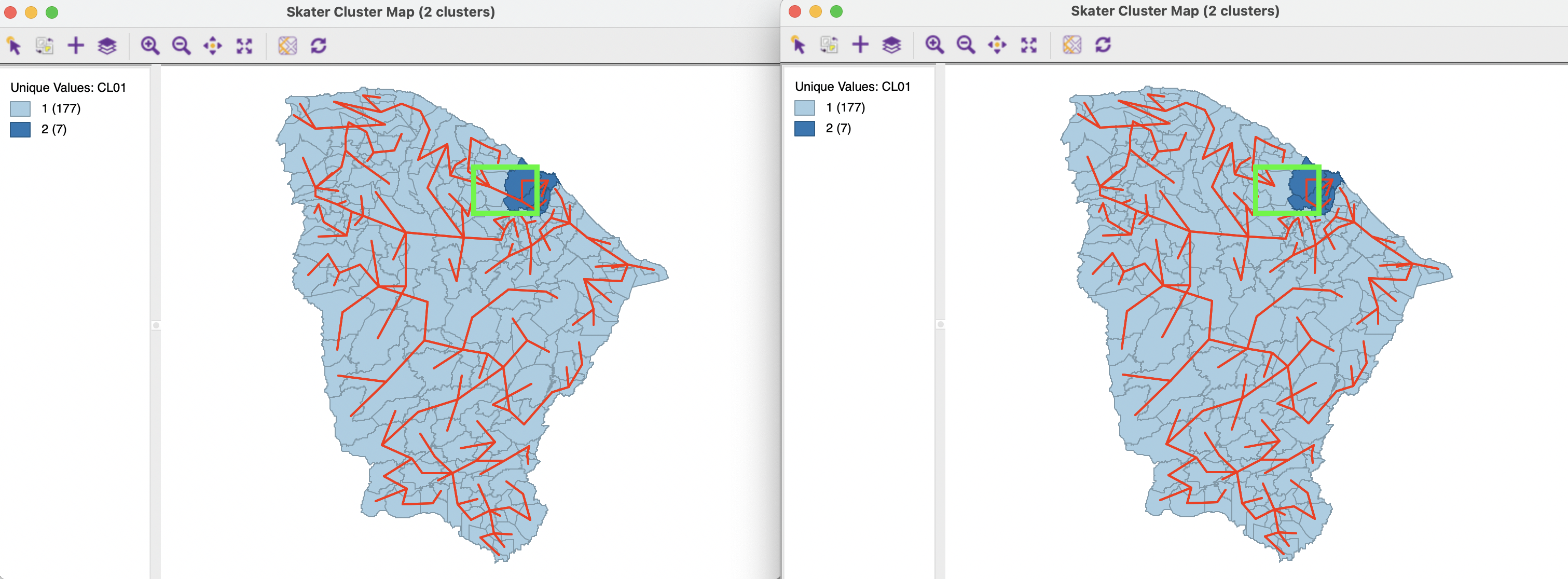
Figure 10.17: Ceará, first cut in MST
To compare the results with the other techniques, Figure 10.18 shows the resulting clusters for \(k\)=12. As was the case for SCHC, the layout is characterized by several singletons, and all but three clusters have fewer than five observations.
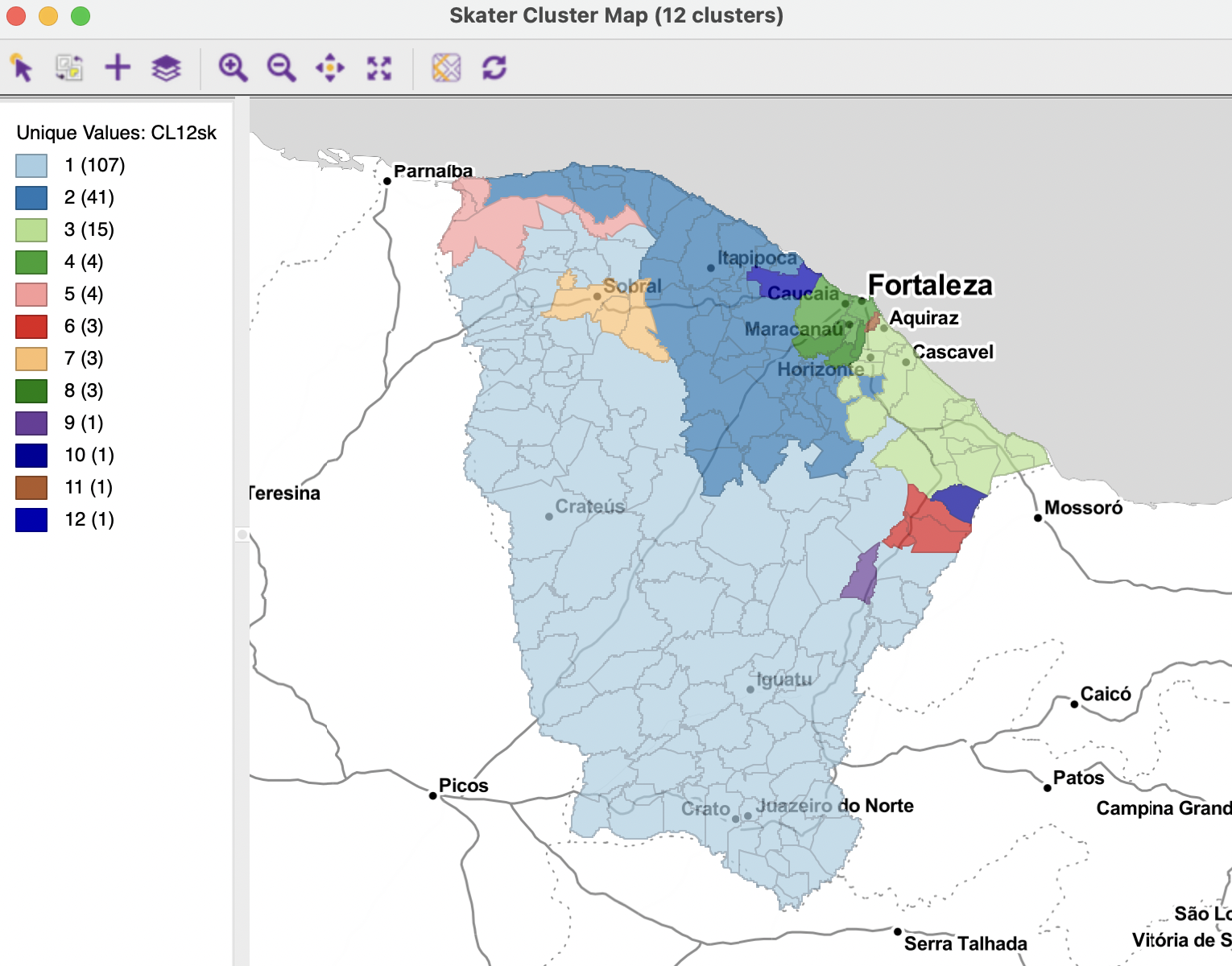
Figure 10.18: Ceará, SKATER cluster map, k=12
The overall characteristics of the SKATER result are slightly worse than for SCHC, as depicted in Figure 10.19. The BSS/TSS ratio of 0.4325 is slightly smaller than the 0.4641 for SCHC (compared to 0.682 for unconstrained K-means).
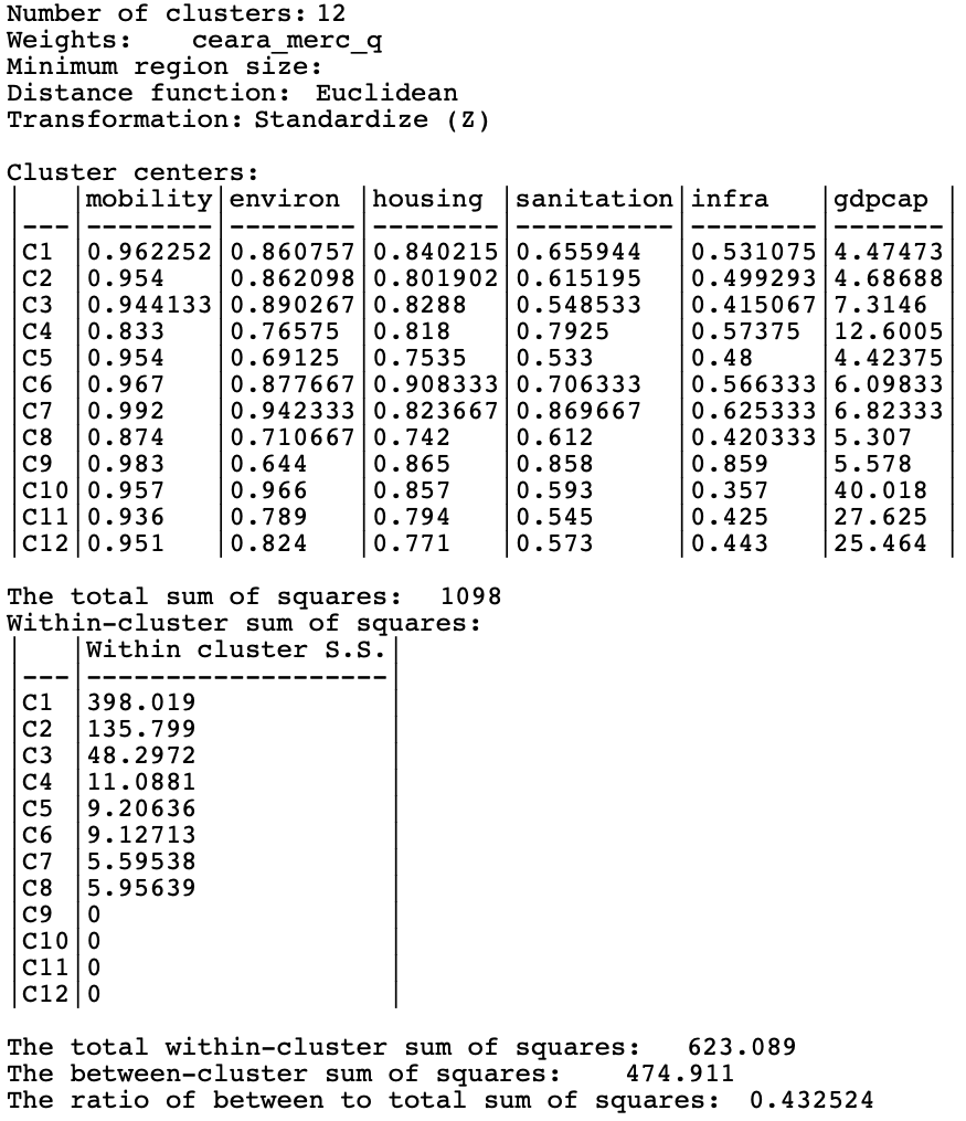
Figure 10.19: Ceará, SKATER cluster characteristics, k=12
10.3.2.1 Saving the Minimum Spanning Tree
Figure 10.17 has the graph structure of the MST visualized on the map. In GeoDa,this is implemented as a special application of the Connectivity property associated with any map window
(see Volume 1), with the weights file that corresponds to the MST selected (active) in the Weights Manager interface.
The MST connectivity structure is saved by means of the Save Spanning Tree option in the Skater Settings dialog. One option is to save the Complete Spanning Tree (select the corresponding box). The default is to save the MST that corresponds with the current solution, i.e., with the edges removed that follow from the various cuts up to that point.
In Figure 10.17, the full MST is shown in the map on the left, whereas the map on the right shows the MST with one edge removed.
10.3.2.2 Setting a minimum cluster size
In some applications of spatially constrained clustering, the resulting regions must satisfy a minimum size requirement. This was discussed in the context of K-means clustering in Section 6.3.4.4. The same option is available here.
There are again two ways to implement the bound. One is based on an spatially extensive variable, like population size. The default is to take the value that corresponds with the 10 percentile, but this does not always lead to feasible solutions. Unlike what is the case for K-means and other not spatially constrained methods, there can be a conflict between the contiguity constraint and the minimum bounds. This is a specific problem for the SKATER algorithm, where solutions for a higher value of \(k\) are always subsets of previous solutions. If the resulting subtree does not meet the minimum bound, there is a conflict between the specified \(k\) and the desired minimum bound.
The same problem holds for the second minimum bound option, i.e. setting a Min Region Size, i.e., the minimum number of observations in each cluster.
For example, with the minimum population set to the 10 percentile of 845,238, it is not possible to obtain seven clusters. As the cluster map in Figure 10.20 shows, the result only shows six clusters, with the smallest consisting of seven observations. The cluster characteristics suffer from the minimum bound constraint, yielding a dismal BSS/TSS ratio of 0.2231.
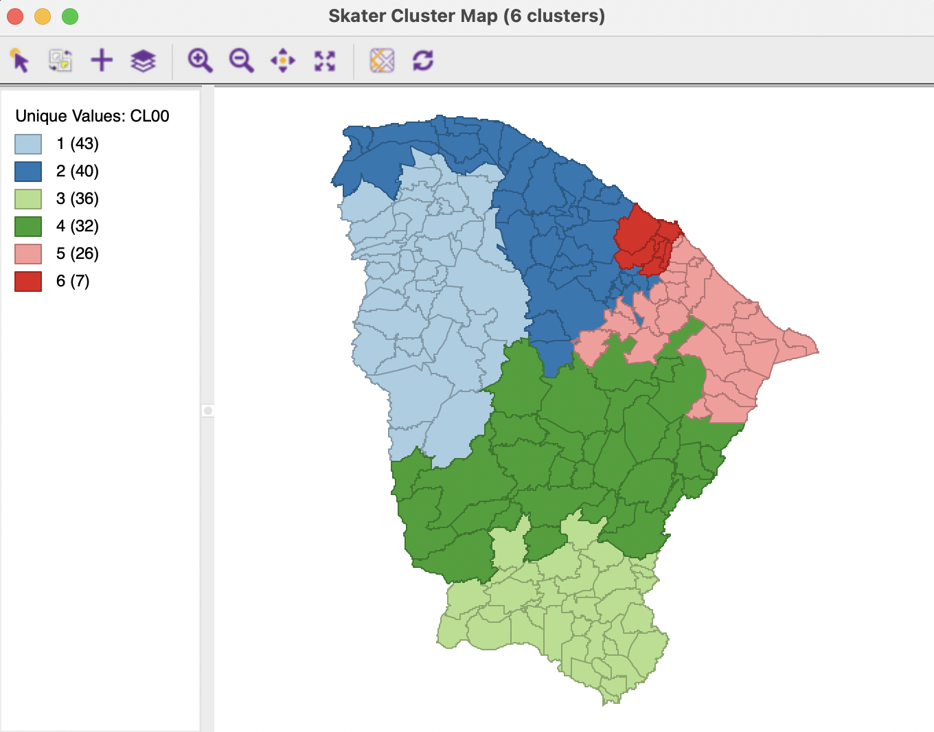
Figure 10.20: Ceará, constrained SKATER cluster map, k=7 with min population size
On the other hand, with a minimum cluster size set to 10, a solution is found for \(k\)=12, shown in Figure 10.21. The results are much more balanced than the unconstrained solution, with half of the clusters containing 10-12 observations. However, the price paid for this constraint is again a substantial deterioration of the BSS/TSS ratio, to 0.266. Also, this constraint breaks down for values of \(k\) of 15 and higher.
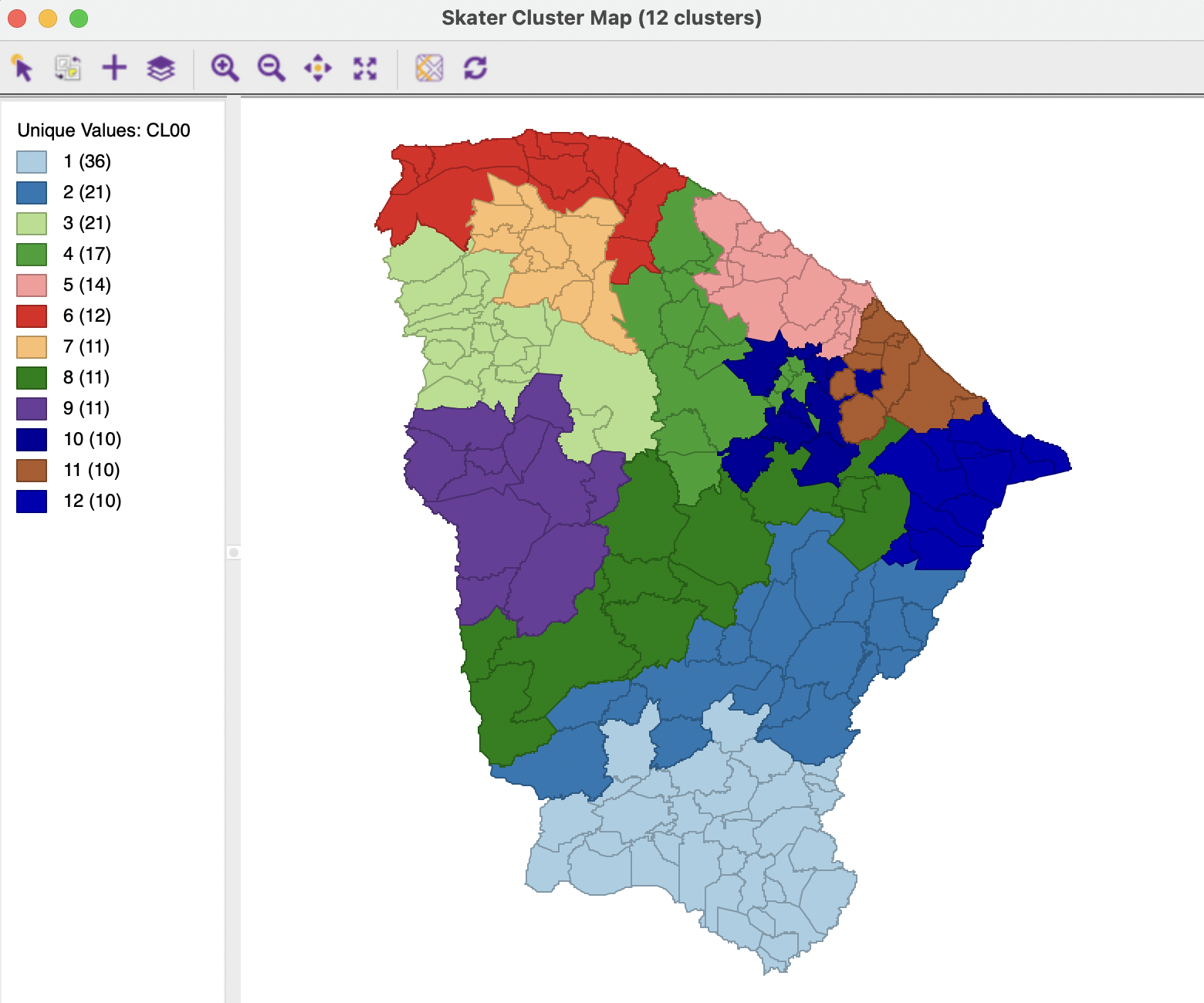
Figure 10.21: Ceará, constrained SKATER cluster map, k=12 with min cluster size 10
This skater algorithm is not to be confused with tools to interpret the results of deep learning https://github.com/oracle/Skater.↩︎
This can readily be computed as \(\sum_i x_i^2 - n_T \bar{x}_T^2\), where \(\bar{x}_T\) is the average for the subtree, and \(n_T\) is the number of nodes in the subtree.↩︎
While this exhaustive evaluation of all potential cuts is inherently slow, it can be sped up by exploiting certain heuristics, as described in Assunção et al. (2006). In
GeoDa, full enumeration is used, but implemented with parallelization to obtain better performance.↩︎Since the variable is standardized, the estimated variance \(\hat{\sigma}^2 = \sum_i x_i^2 / (n - 1) = 1\). Therefore, \(\sum_i x_i^2 = n - 1\), or 13.↩︎