6.2 The K Means Algorithm
As in the case of hierarchical clustering, the point of departure is the sum of dissimilarities between all pairs of observations, which can be separated into a component for within dissimilarity and a component for between dissimilarity: \[T = (1/2) (\sum_{h=1}^k [ \sum_{i \in h} \sum_{j \in h} d_{ij} + \sum_{i \in h} \sum_{j \notin h} d_{ij}]) = W + B.\] As before, \(W\) and \(B\) are complementary, so the lower \(W\), the higher \(B\), and vice versa.
Partitioning methods differ in terms of how the dissimilarity \(d_{ij}\) is defined and how the term \(W\) is minimized. Complete enumeration of all the possible allocations is unfeasible except for toy problems. There is no analytical solution.
The problem is NP-hard, so the solution has to be approached by means of a heuristic, as an iterative descent process. This is accomplished through an algorithm that changes the assignment of observations to clusters so as to improve the objective function at each step. All feasible approaches are based on what is called iterative greedy descent. A greedy algorithm is one that makes a locally optimal decision at each stage. It is therefore not guaranteed to end up in a global optimum, but may get stuck in a local one instead. The optimization strategy is based on an iterative relocation heuristic.
The K-means algorithm uses the squared Euclidean distance as the measure of dissimilarity: \[d_{ij}^2 = \sum_{v=1}^p (x_{iv} - x_{jv})^2 = ||x_i - x_j||^2,\] where the customary notation has been adjusted to designate the number of variables/dimensions as \(p\) instead of \(k\) (since \(k\) is traditionally used for the number of clusters).
This gives the overall objective as finding the allocation \(C(i)\) of each observation \(i\) to a cluster \(h\) out of the \(k\) clusters so as to minimize the within-cluster similarity over all \(k\) clusters: \[\mbox{min}(W) = \mbox{min} (1/2) \sum_{h=1}^k \sum_{i \in h} \sum_{j \in h} ||x_i - x_j||^2,\] where, in general, \(x_i\) and \(x_j\) are \(p\)-dimensional vectors.
A little bit of algebra shows how this simplifies to minimizing the squared difference between the values of the observations in each cluster and the corresponding cluster mean: \[\mbox{min}(W) = \mbox{min} \sum_{h=1}^k n_h \sum_{i \in h} (x_i - \bar{x}_h)^2.\] In other words, minimizing the sum of (one half) of all squared distances is equivalent to minimizing the sum of squared deviations from the mean in each cluster, the within sum of squared errors.
Mathematical details
The objective function is one half the sum of the squared Euclidean distances for each cluster between all the pairs \(i-j\) that form part of the cluster \(h\), i.e., for all \(i \in h\) and \(j \in h\): \[W = (1/2) \sum_{h=1}^k \sum_{i \in h} \sum_{j \in h} ||x_i - x_j||^2 ,\] where, to keep the notation simple, the \(x\) are taken as univariate (without loss of generality).
For each \(i\) in a given cluster \(h\), the sum of the squared distances to all the \(j\) in the cluster is: \[\sum_{j} (x_i - x_j)^2 = \sum_{j} (x_i^2 - 2x_ix_j + x_j^2),\]
dropping the \(\in h\) notation for simplicity.
With \(n_h\) observations in cluster \(h\), \(\sum_j x_i^2 = n_h x_i^2\) (since \(x_i\) does not contain the index \(j\) and thus is simply repeated \(n_h\) times). Also, \(\sum_j x_j = n_h \bar{x}_h\), where \(\bar{x}_h\) is the mean of \(x\) for cluster \(h\). As a result: \[\sum_{j} (x_i - x_j)^2 = n_h x_i^2 - 2 n_h x_i \bar{x}_h + \sum_j x_j^2.\]
Next, using the same approach as for \(j\), and since \(\sum_j x_j^2 = \sum_i x_i^2\), the sum over all \(i\) becomes: \[\sum_i \sum_{j} (x_i - x_j)^2 = n_h \sum_i x_i^2 - 2 n_h^2 \bar{x}_h^2 + n_h \sum_i x_i^2 = 2n_h^2 (\sum_i x_i^2 / n_h - \bar{x}_h^2).\]
Finally, since \(\sum_i x_i^2 / n_h - \bar{x}_h^2 = (1/n_h) \sum_i (x_i - \bar{x}_h)^2\) (the definion of variance), the contribution of cluster \(h\) to the objective function becomes: \[(1/2) \sum_i \sum_{j} (x_i - x_j)^2 = n_h [ \sum_i (x_i - \bar{x}_h)^2 ].\]
For all the clusters jointly, this is simply summed over \(h\).
6.2.1 Iterative Relocation
The K-means algorithm is based on the principle of iterative relocation. In essence, this means that after an initial solution is established, subsequent moves (i.e., allocating observations to clusters) are made to improve the objective function. This is a greedy algorithm, that ensures that at each step the total within-cluster sums of squared errors (from the respective cluster means) is lowered. The algorithm stops when no improvement is possible. However, this does not ensure that a global optimum is achieved (for an early discussion, see Hartigan and Wong 1979). Therefore sensitivity analysis is essential. This is addressed by trying many different initial allocations (typically assigned randomly).
To illustrate the logic behind the algorithm, the same simple toy example as in Chapter 5 is employed. The seven observations are shown in Figure 6.2, with the center (the mean of X and the mean of Y) shown in a lighter color. In K-means, the initial center is not one of the observations. The objective is to group the seven points into two clusters.
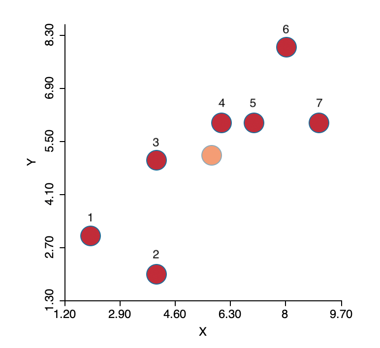
Figure 6.2: K-means toy example
The coordinates of the seven points are given in the X and Y columns of Figure 6.3. The column labeled as SSE shows the squared distance from each point to the center of the point cloud, computed as the average of the X and Y coordinates (X=5.714, Y=5.143).30 The sum of the squared distances constitutes the total sum of squared errors, or TSS, which equals 62.286 in this example. This value does not change with iterations, since it pertains to all the observations taken together and ignores the cluster allocations.
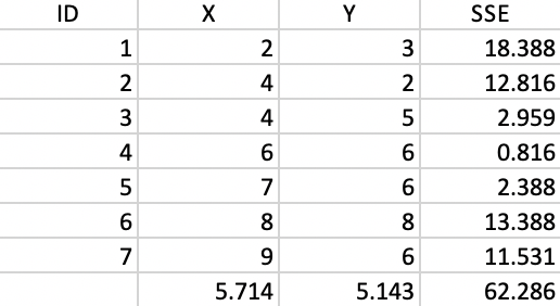
Figure 6.3: Worked example - basic data
The initial step of the algorithm is to randomly pick two seeds, one for each cluster. The seeds are actual observations, not some other random location. In the example, observations 4 and 7 are selected, shown by the lighter color in the upper left panel of Figure 6.4. The other observations are allocated to the cluster whose seed they are closest to.
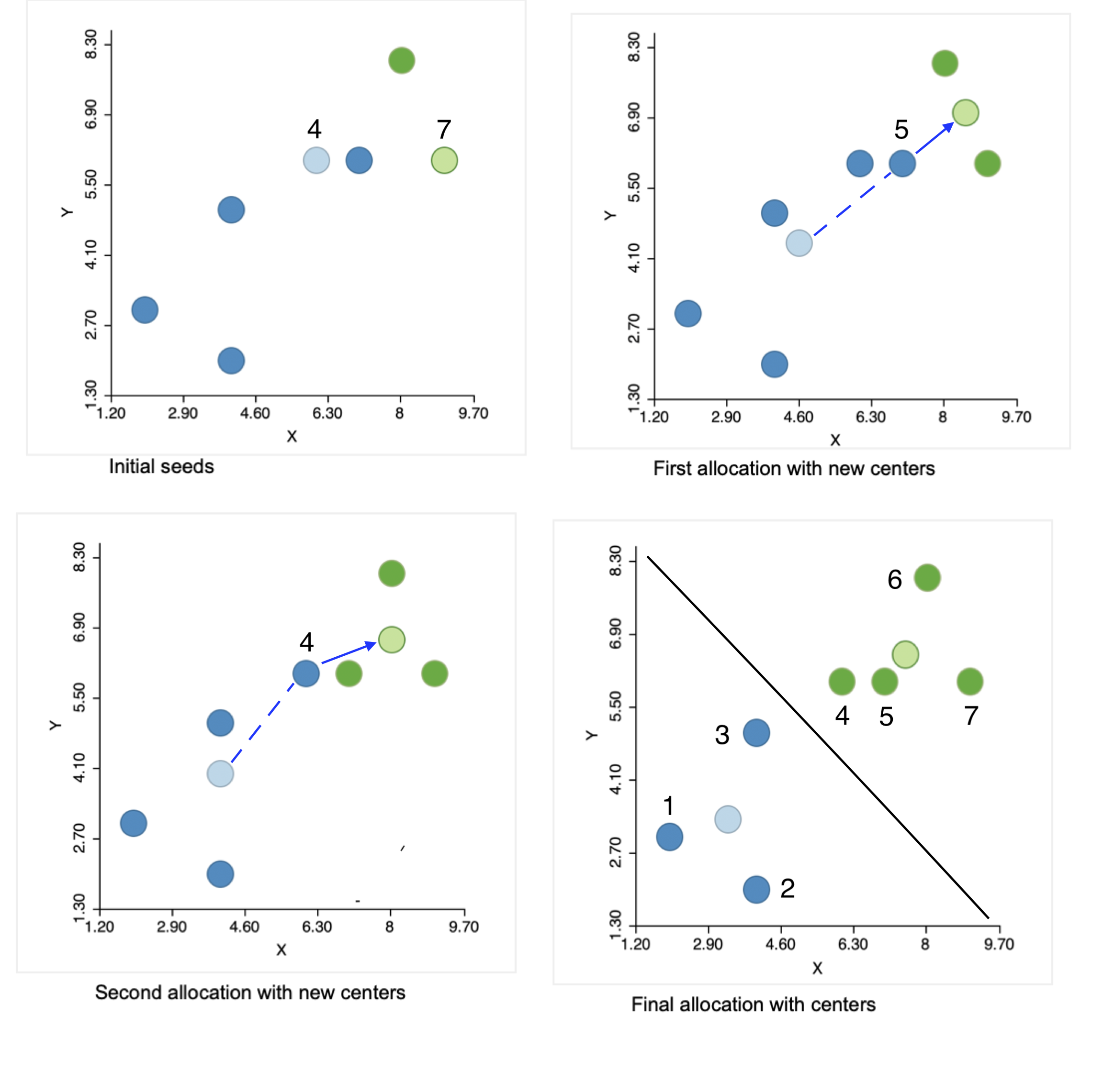
Figure 6.4: Steps in the K-means algorithm
The allocation of observations to the cluster center they are closest to requires the distance from each point to the two seeds. The columns d_i4 and d_i7 in Figure 6.5 contain those respective distances. The highlighted values indicate how the first allocation consists of five observations in cluster 1 (1-5) and two observations in cluster 2 (6 and 7). They are given blue and green colors in the upper left panel of Figure 6.4.
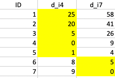
Figure 6.5: Squared distance to seeds
To each of the initial clusters corresponds a new central point, computed as the average of the respective X and Y coordinates, respectively (6.8, 17) and (8.5, 7). The SSE follows as the squared distance between each observation in the cluster and its central point, as listed in Figure 6.6. The sum of the total SSE in each cluster is the within sum of squares, WSS = 28.4 + 2.5 = 30.9 in this first step. Consequently, the between sum of squares BSS = TSS - WSS = 62.3 - 30.9 = 31.4. The associated ratio BSS/TSS, an indicator of the quality of the cluster, is 0.50.
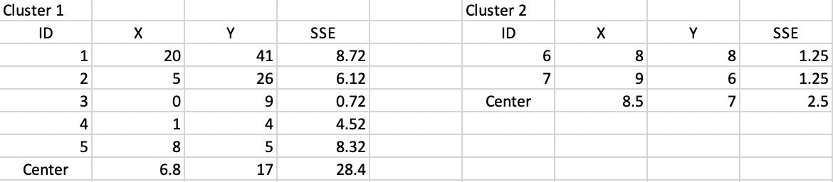
Figure 6.6: Step 1 - Summary characteristics
With the new cluster center points in place, each observation is again allocated to the closest center. From the calculations in Figure 6.7, this results in observation 5 moving from cluster 1 to cluster 2, which now consists of three observations (cluster 1 has the remaining four). This move is illustrated in the upper right panel of Figure 6.4.
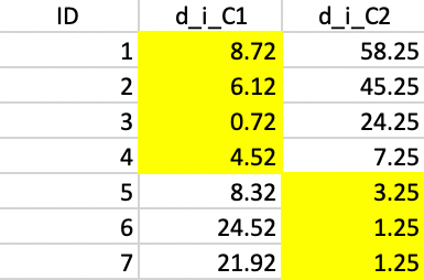
Figure 6.7: Squared distance to Step 1 centers
The new clusters yield cluster centers at (4, 4) and (8, 6.667). The associated SSE are shown in Figure 6.8. This results in an updated WSS of 18 + 4.667 = 22.667, clearly an improvement of the objective function (down from 30.9). The corresponding ratio of BSS/TSS becomes 0.64, also a substantial improvement relative to 0.50.
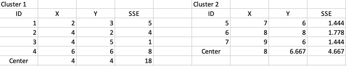
Figure 6.8: Step 2 - Summary characteristics
Figure 6.9 lists the distances for each point to the new cluster centers. This results in observation 4 moving from cluster 1 to cluster 2, shown in the lower left panel of Figure 6.4.
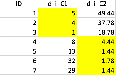
Figure 6.9: Squared distance to Step 2 centers
The new cluster centers are (3.333, 3.333) and (7.5, 6.5). The associated SSE are shown in Figure 6.10, with a WSS of 7.333 + 8 = 15.333 and an associated BSS/TSS of 0.75. This latest allocation no longer results in a change, yielding a local optimum, illustrated in the lower-right panel in Figure 6.4..
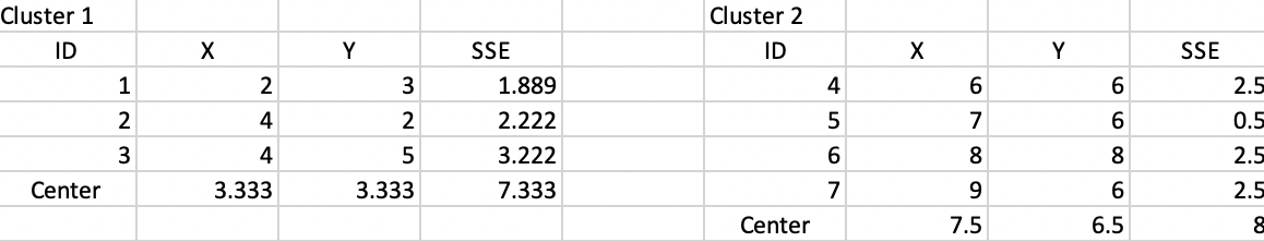
Figure 6.10: Step 3 - Summary characteristics
This solution corresponds to the allocation that would result from a Voronoi diagram or Thiessen polygon around the cluster centers. All observations are closer to their center than to any other center. This is indicated by the black line in the graph, which is perpendicular at the midpoint to an imaginary line connecting the two centers and separates the area into two compact regions.
6.2.2 The Choice of K
A key element in the K-means method is the choice of the number of clusters, \(k\). Typically, several values for \(k\) are considered, and the resulting clusters are then compared in terms of the objective function.
Since the total sum of squared errors (SSE) equals the sum of the within-group SSE and the total between-group SSE, a common criterion is to assess the ratio of the total between-group sum of squares (BSS) to the total sum of squares (TSS), i.e., BSS/TSS. A higher value for this ratio suggests a better separation of the clusters. However, since this ratio increases with \(k\), the selection of a best \(k\) is not straightforward. Several ad hoc rules have been suggested, but none is totally satisfactory.
One useful approach is to plot the objective function against increasing values of \(k\). This could be either the within sum of squares (WSS), a decreasing function with \(k\), or the ratio BSS/TSS, a value that increases with \(k\). The goal of a so-called elbow plot is to find a kink in the progression of the objective function against the value of \(k\) (see Section 6.3.4.2). The rationale behind this is that as long as the optimal number of clusters has not been reached, the improvement in the objective should be substantial, but as soon as the optimal \(k\) has been exceeded, the curve flattens out. This is somewhat subjective and often not that easy to interpret in practice. GeoDa’s functionality does not include an elbow plot, but all the information regarding the objective functions needed to create such a plot is provided in the output. This is illustrated in Section 6.3.4.2.
A more formal approach is the so-called Gap statistic of Tibshirani, Walther, and Hastie (2001), which employs the difference between the log of the WSS and the log of the WSS of a uniformly randomly generated reference distribution (uniform over a hypercube that contains the data) to construct a test for the optimal \(k\). Since this approach is computationally quite demanding, it is not further considered.
6.2.3 K-means++
Typically, the assignment of the first set of \(k\) cluster centers is obtained by uniform random sampling \(k\) distinct observations from the full set of \(n\) observations. In other words, each observation has the same probability of being selected.
The standard approach is to try several random assignments and start with the one that gives the best value for the objective function (e.g., the smallest WSS, or the largest BSS/TSS). This is one of the two approaches implemented in GeoDa. In order to ensure that the results are reproducible, it
is important to set a seed value for the random number generator. Also, to further assess the
sensitivity of the result to the starting point, different seeds should be tried (as well as a
different number of initial solutions).31
A second approach uses a careful consideration of initial seeds, following the procedure outlined in Arthur and Vassilvitskii (2007), commonly referred to as K-means++. The rationale behind K-means++ is that rather than sampling uniformly from the \(n\) observations, the probability of selecting a new cluster seed is changed in function of the distance to the nearest existing seed. Starting with a uniformly random selection of the first seed, say \(c_1\), the probabilities for the remaining observations are computed as: \[p_{j \neq c_1} = \frac{d_{jc_1}^2}{\sum_{j \neq c_1} d_{jc_1}^2 }.\] In other words, the probability is no longer uniform, but changes with the squared distance to the existing seed: the smaller the distance, the smaller the probability. This is referred to by Arthur and Vassilvitskii (2007) as the squared distance (\(d^2\)) weighting.
The weighting increases the chance that the next seed is further away from the existing seeds, providing a better coverage over the support of the sample points. Once the second seed is selected, the probabilities are updated in function of the new distances to the closest seed, and the process continues until all \(k\) seeds are picked.
While generally being faster and resulting in a superior solution in small to medium sized data sets, this method does not scale well (as it requires \(k\) passes through the whole data set to recompute the distances and the updated probabilities). Also, a choice of a large number of random initial allocations may yield a better outcome than the application of K-means++, at the expense of a somewhat longer execution time.
Each squared distance is \((x_i - \bar{x})^2 + (y_i - \bar{y})^2\).↩︎
GeoDaimplements this approach by leveraging the functionality contained in the C Clustering Library (de Hoon, Imoto, and Miyano 2017).↩︎