3.2 Classic Metric Scaling
Multidimensional Scaling or MDS is a classic multivariate approach designed to portray the embedding of a high-dimensional data cloud in a lower dimension, typically 2D or 3D. The technique goes back to pioneering work on so-called metric scaling by Torgerson (Torgerson 1952, 1958), and its extension to non-metric scaling by Shepard and Kruskal (Shepard 1962a, 1962b; Kruskal 1964). A very nice overview of the principles and historical evolution of MDS as well as a more complete list of the classic references can be found in Mead (1992).
MDS is based on the notion of distance between observation points in multi-attribute space. For \(k\) variables, the Euclidean distance between observations \(x_i\) and \(x_j\) in \(k\)-dimensional space is \[d_{ij} = || x_i - x_j|| = [\sum_{h=1}^k (x_{ih} - x_{jh})^2]^{1/2},\] the square root of the sum of the squared differences between two data points over each variable dimension.
In this expression, \(x_i\) and \(x_j\) are \(k\)-dimensional column vectors, with one value for each of the \(k\) variables (dimensions). In practice, it turns out that working with the squared distance is mathematically more convenient, and it does not affect the properties of the method. In order to differentiate the two notions, the notation \(d_{ij}^2\) will be used for the squared distance.
The squared distance can also be expressed as the inner product of the difference between two vectors: \[d_{ij}^2 = (x_i - x_j)'(x_i - x_j),\] with \(x_i\) and \(x_j\) represented as \(k \times 1\) column vectors. It is important to keep the dimensions straight, since the data points are typically contained in an \(n \times k\) matrix \(X\), where each observation corresponds to a row of the matrix. However, in order to obtain the sum of squared differences as a inner product, each observation (on the \(k\) variables) must be represented as a column vector.
An alternative to Euclidean distance is a Manhattan (city block) distance, which is less susceptible to outliers, but does not lend itself to being expressed as an inner product of two vectors. The corresponding expression is: \[d_{ij} = \sum_{h=1}^k |x_{ih} - x_{jh}|,\] i.e., the sum of the absolute differences in each dimension.
The objective of MDS is to find the coordinates of data points \(z_1, z_2, \dots, z_n\) in 2D or 3D that mimic the distance in multi-attribute space as closely as possible. More precisely, for each observation \(i\) \((i = 1, \dots, n)\), \(z_i\) consists of a pair of coordinates (for 2D MDS), or a triple (for 3D MDS), which need to be found from the original \(k\)-dimensional coordinates.
The problem can be formulated as minimizing a stress function, \(S(z)\): \[S(z) = \sum_i \sum_j (d_{ij} - ||z_i - z_j||)^2.\] In other words, a set of coordinates in a lower dimension (\(z_i\), for \(i = 1, \dots, n\)) are found such that the distances between the resulting pairs of points ( \(||z_i - z_j||\) ) are as close as possible to their pair-wise distances in high-dimensional multi-attribute space ( \(d_{ij}\) ).
Due to the use of a squared difference, the objective of the stress function penalizes large differentials more. Hence, there is a tendency of MDS to represent points that are far apart rather well, but maybe with less attention to points that are closer together. This may not be the best option when attention focuses on local clusters, i.e., groups of observations that are close together in multi-attribute space. An alternative that gives less weight to larger distances is Stochastic Neighbor Embedding (SNE), considered in Chapter 4.
3.2.1 Mathematical Details
Classic metric MDS approaches the optimization problem indirectly by focusing on the cross product between the actual vectors of observations \(x_i\) and \(x_j\) rather than between their difference, i.e., the cross-product between each pair of rows in the observation matrix \(X\). The values for all these cross-products are contained in the matrix expression \(XX'\). This matrix, often referred to as a Gram matrix, is of dimension \(n \times n\), and not \(k \times k\) as is the case for the more familiar \(X'X\) used in PCA.
If the actual observation matrix \(X\) is available, then the eigenvalue decomposition of the Gram matrix provides the solution to MDS. In the same notation as used for PCA (but now pertaining to the matrix \(XX'\)), the spectral decomposition yields: \[XX' = VGV',\] where V is the matrix with eigenvectors (each of dimension \(n \times 1\)) and \(G\) is a \(n \times n\) diagonal matrix that contains the eigenvalues on the diagonal.
Since the matrix \(XX'\) is symmetric, all its eigenvalues are non-negative, so that their square roots exist. The decomposition can therefore also be written as: \[XX' = VG^{1/2}G^{1/2}V' = (VG^{1/2})(VG^{1/2})'.\] In other words, the matrix \(VG^{1/2}\) can play the role of \(X\) as far as the Gram matrix is concerned. It is not the same as \(X\), in fact it is expressed as coordinates in a different (rotated) axis system, but it yields the same distances (its Gram matrix is the same as \(XX'\)). Points in either multidimensional space have the same relative positions.
In practice, to express this in lower dimensions, only the first and second (and sometimes third) columns of \(VG^{1/2}\) are selected. Consequently, only the two/three largest eigenvalues and corresponding eigenvectors of \(XX'\) are required. These can be readily computed by means of the power iteration method.
3.2.1.1 Classic metric MDS and principal components
In Chapter 2, the principal components \(XV\) were shown to equal the product \(UD\) from the SVD of the matrix \(X\). Using the SVD for \(X\), the Gram matrix can also be written as: \[XX' = (UDV')(VDU') = UD^2U',\] since \(V'V = I\). In other words, the role of \(VG^{1/2}\) can also be played by \(UD\), which is the same as the principal components.
More precisely, the first few dimensions of the classic metric MDS will correspond with the first few principal components of the matrix \(X\), associated with the largest eigenvalues (in absolute value). However, the distinguishing characteristic of MDS is that it can be applied without knowing \(X\), as shown in Section 3.2.1.3.
3.2.1.2 Power iteration method
The power method is an iterative approach to obtain the eigenvector associated with the largest eigenvalue of a matrix. It is found from an iteration that starts with an arbitrary unit vector, say \(x_0\).9 For any given matrix \(A\), the first step is to obtain a new vector as the product of the initial vector and the matrix \(A\), \(x_1 = A x_0\). The procedure iterates by applying higher and higher powers to the transformation \(x_{k} = A x_{k-1} = A^k x_{0}\), until convergence (i.e., the difference between \(x_k\) and \(x_{k-1}\) is less than a pre-defined threshold). The end value, \(x_k\), is a good approximation to the dominant eigenvector of \(A\).10
The associated eigenvalue is found from the so-called Rayleigh quotient: \[\lambda = \frac{x_k' A x_k}{x_k ' x_k}.\]
The second largest eigenvector is found by applying the same procedure to the matrix \(B\), where \(B\) can be viewed as some sort of residual after the result for the largest eigenvector has been applied: \[B = A - \lambda x_k x_k'.\] The idea can be extended to obtain more eigenvalues/eigenvectors, although typically the power method is only used to compute a few of the largest ones. The procedure can also be applied to the inverse matrix \(A^{-1}\) to obtain the smallest eigenvalues.
3.2.1.3 Dissimilarity matrix
The reason why the solution to the metric MDS problem can be found in a fairly straightforward analytic way has to do with the interesting relationship between the squared distance matrix and the Gram matrix for the observations, the matrix \(XX'\). Note that this only holds for Euclidean distances. As a result, the Manhattan distance option is not available for the classic metric MDS.
The squared Euclidean distance between two points \(i\) and \(j\) in \(k\)-dimensional space is: \[d^2_{ij} = \sum_{h=1}^k (x_{ih} - x_{jh})^2,\] where \(x_{ih}\) corresponds to the \(h\)-th value in the \(i\)-th row of \(X\) (i.e., the \(i\)-th observation), and \(x_{jh}\) is the same for the \(j\)-th row. After working out the individual terms of the squared difference, this becomes: \[d^2_{ij} = \sum_{h=1}^k (x_{ih}^2 + x_{jh}^2 - 2 x_{ih}x_{jh}).\]
The full matrix \(D^2\) for all pairwise distances between observations for a given variable (column) \(h\) simply contains the corresponding term in each position \(i-j\). It turns out that the squared distance matrix between all pairs of observations for a given variable \(h\) can then be written as: \[D^2_h = c_{h} \iota' + \iota c_{h}' - 2 x_{h} x_{h}',\] with \(c_{h} = x_{ih}^2\), the square of the variable \(h\) at each location, and \(\iota\) as a \(n \times 1\) vector of ones.
The full \(n \times n\) squared distance matrix consists of the sum of the individual squared distance matrices over all variables/columns: \[D^2 = c \iota' + \iota c' - 2 XX',\]
since \(\sum_{h = 1}^k x_h x_h' = XX'\), and with each element of \(c = \sum_{h=1}^k x_{ih}^2\), for \(i = 1, \dots, n\).
This establishes an important connection between the squared distance matrix and the Gram matrix. After some matrix algebra, the relation between the two matrices can be established as: \[XX' = - \frac{1}{2} (I - M)D^2(I - M),\] where \(M\) is the \(n \times n\) matrix \((1/n)\iota \iota'\) and \(\iota\) is a \(n \times 1\) vector of ones (so, \(M\) is an \(n \times n\) matrix containing 1/n in every cell). The matrix \((I - M)\) converts values into deviations from the mean. In the literature, the joint pre- and post-multiplication by \((I - M)\) is referred to as double centering.
Given this equivalence, the matrix of observations \(X\) is not actually needed (in order to construct \(XX'\)), since the eigenvalue decomposition can be applied directly to the double centered squared distance matrix.11
3.2.2 Implementation
Classic metric MDS is invoked from the drop down list created by the toolbar Clusters icon (Figure 3.1) as the second item (more precisely, the second item in the dimension reduction category). Alternatively, from the main menu, Clusters > MDS gets the process started.
The same ten community bank efficiency characteristics are used as in the treatment of principal components in Chapter 2. They are listed again for easy of interpretation:
- CAPRAT: ratio of capital over risk weighted assets
- Z: z score of return on assets (ROA) + leverage over the standard deviation of ROA
- LIQASS: ratio of liquid assets over total assets
- NPL: ratio of non-performing loans over total loans
- LLP: ratio of loan loss provision over customer loans
- INTR: ratio of interest expense over total funds
- DEPO: ratio of total deposits over total assets
- EQLN: ratio of total equity over customer loans
- SERV: ratio of net interest income over total operating revenues
- EXPE: ratio of operating expenses over total assets
The process is started with the MDS Settings dialog, shown in Figure 3.2. This is where the variables and various options are selected. For now, everything is kept to the default settings, with Method as classic metric and the # of Dimensions set to 2. The variables are used in standardized form (Transformation is set to Standardize (Z)), with the usual set of alternative transformations available as options.
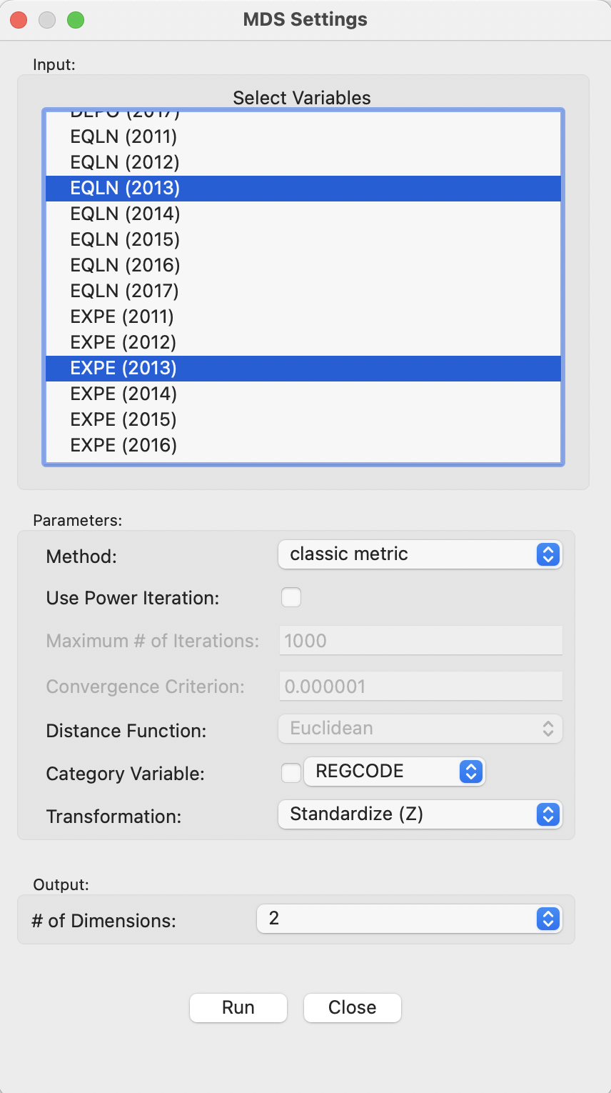
Figure 3.2: MDS Main Dialog
3.2.2.1 Saving the MDS coordinates
After the Run button is pressed, a small dialog appears to select the variables for the MDS dimensions, i.e., the new x and y axes for a two-dimensional MDS. The default variable names are V1 and V2. With the variable names selected, the new values are added to the data table and the MDS scatter plot is shown, as in Figure 3.3.
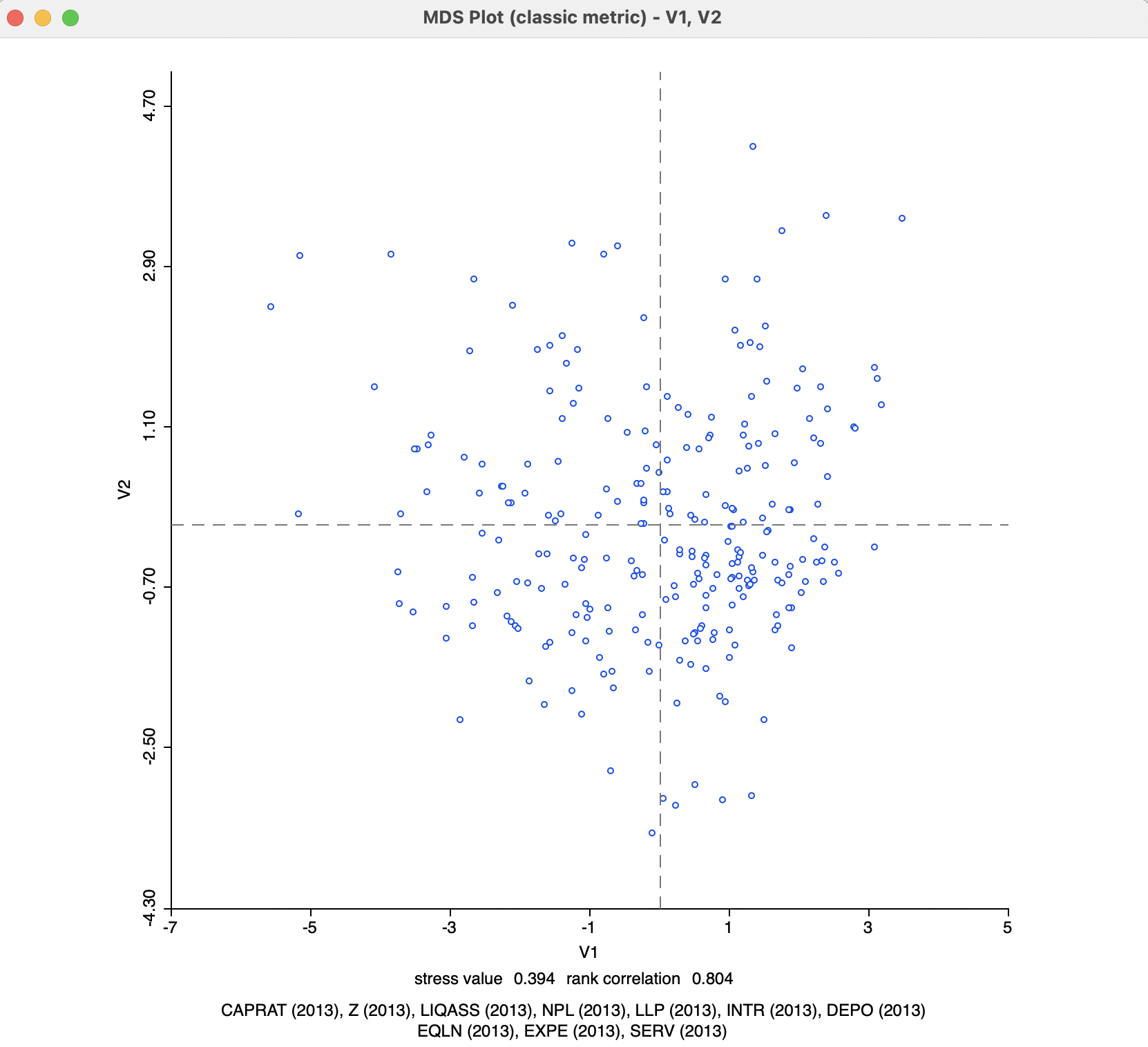
Figure 3.3: MDS Scatter Plot - Default Settings
Below the scatter plot are two lines with statistics. They can be removed by turning the option View > Statistics off (the default is on). The variables that were used in the analysis are listed, as well as two measures of fit, the stress value and the rank correlation. The stress value gives an indication of how the objective function is met, with smaller values indicating a better fit. The rank correlation is between the original inter-observation distances and the distances in the MDS plot. Here, higher values indicate a better fit. In the example, the results are 0.394 for the stress value and 0.804 for the rank correlation, suggesting a reasonable performance.
3.2.2.2 MDS and PCA
The MDS scatter plot obtained from the classic metric method is essentially the same as the scatter plot of the two first principal components, shown in Figure 2.9. Figure 3.4 indicates how one is the mirror image of the other (flipped around the y-axis). In other words, points in the MDS scatter plot that are close together correspond to points that are close together in the PCA scatter plot.
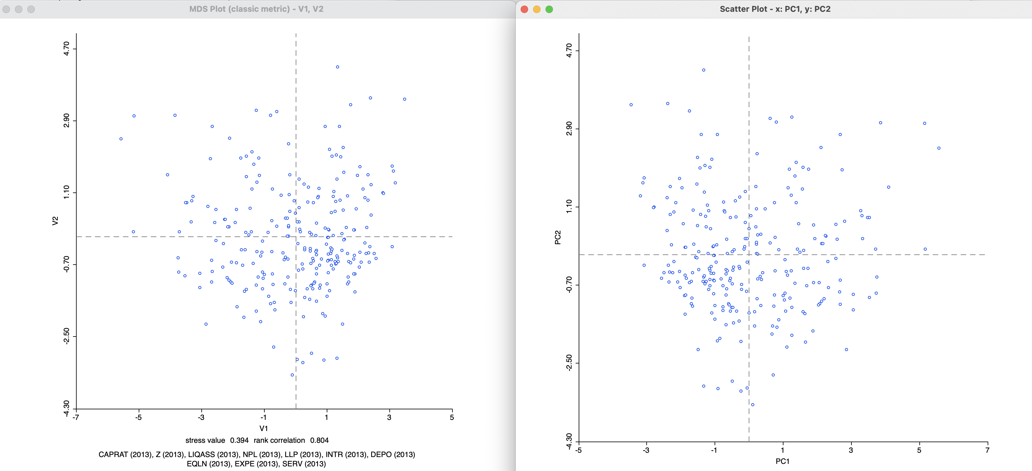
Figure 3.4: MDS and PCA Scatter Plot
The equivalence between the two approaches is further illustrated in Figure 3.5, where the values for the x-coordinates in both plots are graphed against each other. There is a perfect negative relationship between the two, i.e., they are identical, except for the sign.
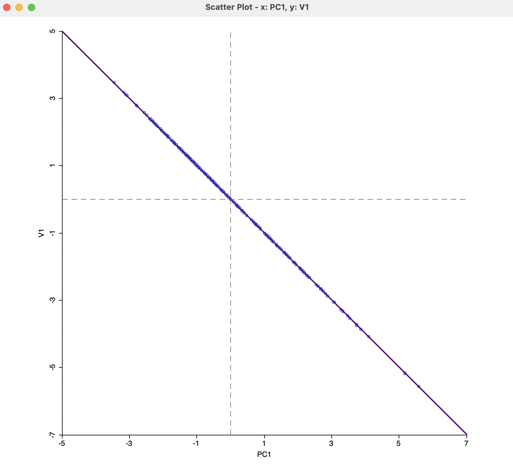
Figure 3.5: MDS Dimensions and PCA
3.2.2.3 Power approximation
An option that is particularly useful in larger data sets is to use a Power Iteration to approximate the first few largest eigenvalues needed for the MDS algorithm. Since the first two or three eigenvalue/eigenvector pairs are all that is needed for the classic metric implementation, this provides considerable computational advantages in large data sets. Recall that the matrix for which the eigenvalues/eigenvectors need to be obtained is of dimension \(n \times n\). For large \(n\), the standard eigenvalue calculation will tend to break down.
The Power Iteration option is selected by checking the corresponding box in the Parameters panel of Figure 3.2. This also activates the Maximum # of Iterations option. The default is set to 1000, which should be fine in most situations. However, if needed, it can be adjusted by entering a different value in the corresponding box.
In this example, there is no noticeable difference between the standard solution and the power approximation, as illustrated by the scatter plot in Figure 3.6. However, for data sets with several thousands of observations, the power approximation may offer the only practical option to compute the leading eigenvalues.
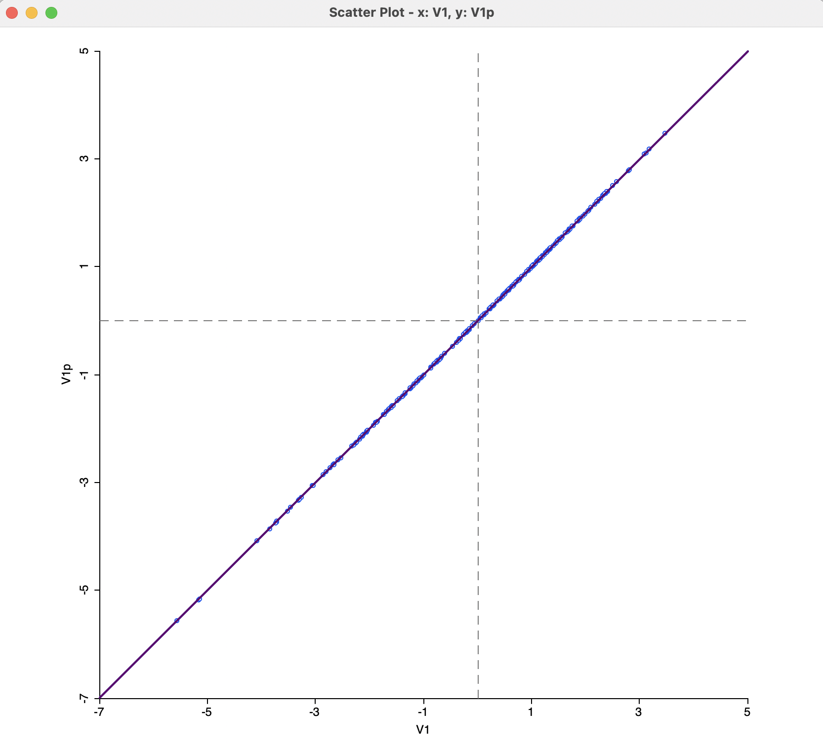
Figure 3.6: MDS Power Approximation
Other options to visualize the results of MDS as well as spatialization of the MDS analysis are further considered in Sections 3.4 and 3.5.
\(x_0\) is typically a vector of ones divided by the square root of the dimension. So, if the dimension is \(n\), the value would be \(1/\sqrt{n}\).↩︎
For a formal proof, see, e.g., Banerjee and Roy (2014), pp. 353-354.↩︎
A more formal explanation of the mathematical properties can be found in Borg and Groenen (2005), Chapter 7, and Lee and Verleysen (2007), pp. 74-78.↩︎