12.3 External Validity

External validity measures are designed to compare a clustering result to an underlying truth, typically carried out through experiments on artificial data sets (see, e.g., Meila 2015; Aydin et al. 2021). However, such indices can also be employed to assess how much different clustering methods result in classifications that are similar in some respects. In general, the clusterings may be for different number of clusters, but for simplicity, only the case where \(k\) is the same in both classifications is taken into account.

Two categories of measures are considered here. First, two classic measures of external validity are considered, i.e., the Adjusted Rand Index (ARI) and the Normalized Information Distance (NID). This is followed by some examples of how the linking and brushing capabilities in GeoDa can be used to gain insight into the overlap between clusters, including by means of the specialized cluster match map.

12.3.1 Classic Measures

12.3.1.1 Adjusted Rand Index

Classic external validity measures can be categorized into pair counting based methods and information theoretic measures. Arguably the most commonly used index based on the former is the Adjusted Rand Index (ARI), originally suggested by Hubert and Arabie (1985).

The ARI is derived by classifying the number of pairs of observations in terms of the extent to which they belong to common clusters. More precisely, all pairs of observations in two clusterings are considered, e.g., clusters labeled \(P\) and \(V\). The pairs are classified into four categories: \(N_{11}\), the number of pairs in the same cluster in both classifications; \(N_{00}\) the number of pairs in different clusters in both classifications; \(N_{01}\) the pairs in the same cluster in \(P\), but in different clusters in \(V\); and \(N_{10}\), the pairs that are in different clusters in \(P\), but in the same cluster in \(V\).

The Adjusted Rand Index (ARI) is then defined as: \[ARI(P,V) = \frac{2N_{00}N_{11} - N_{01}N_{10}}{(N_{00} + N_{01})(N_{01} + N_{11}) + (N_{00}+N_{10})(N_{10}+N_{11})}\] This index is calibrated such that the maximum value is 1. The measure is symmetric, so that the ARI of P relative to V is the same as that of V relative to P.

For the Ceará example, the results of each pairwise ARI are listed in Figure 12.6. There is a clear split between the match of the non-spatial methods and that of the spatially constrained clusters. The former yield an ARI of 0.352, more than double the value for any non-spatial/spatial pair. The spatially constrained clusters are more similar among themselves, with the closest match between SCHC and REDCAP for an ARI of 0.910. Other close matches are between REDCAP and AZP-init (0.700), and SCHC and AZP-init (0.677). The lowest values are between the non-spatial clusters and SKATER (respectively, 0.062 for K-Means and 0.075 for Hierarchical clustering).

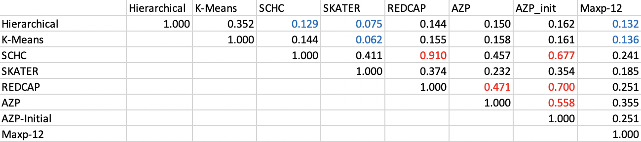
Figure 12.6: Adjusted Rand Index

12.3.1.2 Normalized Information Distance

A second class of methods is based on information theoretic concepts, such as the entropy and mutual information (Vinh, Epps, and Bailey 2010). The entropy is defined above as a measure of the balance in a given cluster result (see Section 12.2.2). A second important concept is the mutual information between clusters \(P\) and \(V\). It is computed as: \[I(P,V) = \sum_{i=1}^k \sum_{j=1}^k \frac{n_{ij}}{n} \log \frac{n_{ij}/n}{n_in_j / n^2},\] where \(n_{ij}\) is the number of observation pairs that are in cluster \(i\) in \(P\) and in cluster \(j\) in \(V\).

The Normalized Information Distance is then obtained as: \[NID = 1 - \frac{I(P,V)}{\mbox{max}(H(P),H(V))},\] where \(H\) is the entropy of a given clustering. The measure is such that lower values suggest a better fit (the minimum is zero).

The results for the Ceará example are shown in Figure 12.7. The relative ranking is essentially the same in qualitative terms as for ARI, with only marginal differences. As before, the best match is between SCHC and REDCAP, and the worst fit between the non-spatial methods and SKATER.

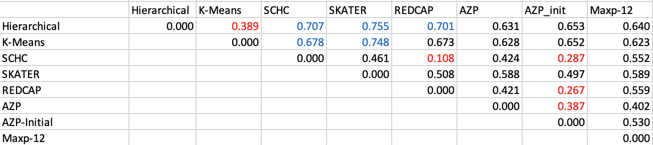
Figure 12.7: Normalized Information Distance

12.3.2 Visualizing Cluster Match

A more informal way to assess the match between cluster results can be obtained by means of the linking and brushing inherent in the mapping functionality. The point of departure is that each cluster classification corresponds to a categorical variable that can be used to create a unique values map.

12.3.2.1 Linking Cluster Maps

With the maps side by side for two clusterings, a category can be selected in one and the matching observations identified in the other. For example, in Figure 12.8, the cluster maps for K-Means and SKATER are shown side-by-side, two clusterings that showed the least correspondence according to ARI and NID. With cluster 1 selected in the K-Means map (the pointer is over the first box in the legend), its 31 observations are highlighted in both maps. One can visually identify the match between the two classifications by locating pairs of observations from cluster 1 for K-Means that are in the same cluster in both maps, and those that are not. For example, the pair highlighted with the blue rectangle are in the same cluster in both classifications (this happens to be labeled cluster 1 in both maps, but that is pure coincidence). In contrast, the pair highlighted with the red rectangle does no longer belong to the same cluster for SKATER (one observation is now in cluster 3 and one in cluster 6).

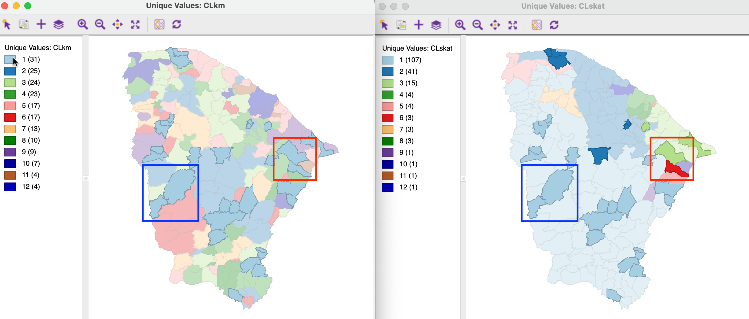
Figure 12.8: K-Means and SKATER overlap

In addition to considering pairs of observations, which follows the pair counting logic, one can also exploit the linking functionality to identify the overlap between clusters as such. For example, in Figure 12.9, the cluster maps are shown for SCHC and REDCAP, the two clusterings that had the closest match using the external validity indices. The cluster maps indeed are highly similar. For example, of the 21 observations in cluster 3 for SCHC, 16 make up cluster 4 for REDCAP. The five remaining observations (highlighted in the red rectangle) are part of cluster 2 for REDCAP (which has 52 observations).

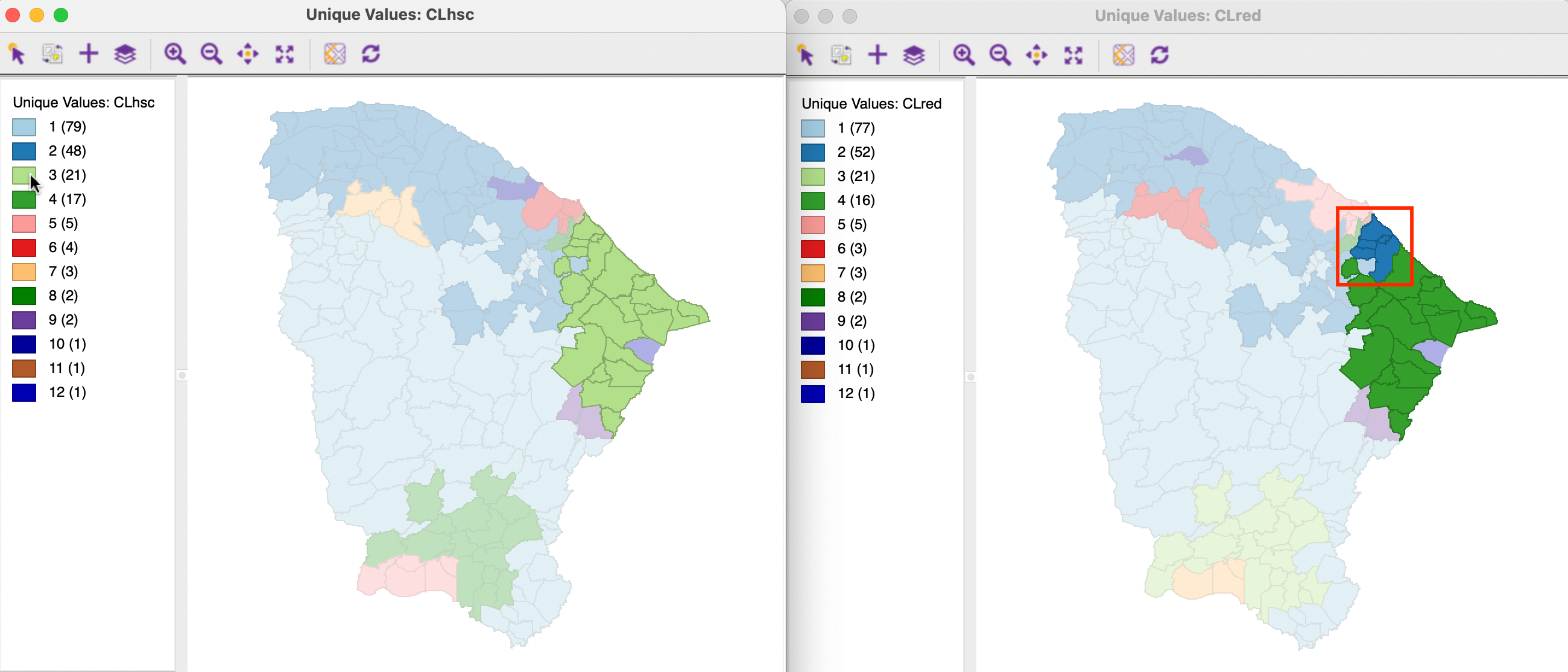
Figure 12.9: SCHC and REDCAP overlap

12.3.2.2 Cluster Match Map

A slightly more automatic approach to visualizing the overlap between different cluster categories is offered by the Cluster Match Map. This function is invoked as Cluster > Cluster Match Map from the menu, or from the cluster toolbar icon drop down list, as shown in Figure 12.1.

The Cluster Match Map Settings dialog requires the selection of the Origin Cluster Indicator and Target Cluster Indicator. For example, the first cluster could be SKATER, with indicator CLskat, and the second cluster K-Means, with indicator CLkm (the reverse of the situation in Figure 12.8). The cluster to compare in the origin cluster is selected by checking the corresponding box. The resulting cluster overlap is by default stored in the variable CL_COM (as usual, this can be changed).

The result for cluster 2 in SKATER (41 observations) is illustrated in Figure 12.10. This is the same outcome as the linked observations in the K-Means cluster map that result from selecting cluster 2 in the SKATER cluster map, but the number of observations in each overlap are listed as well. The cluster label is the label from the target cluster, i.e., K-Means. In addition, the color codes match the codes in the K-Means cluster map classification.

In the example, the 41 observations in cluster 2 of SKATER map into 6 observations in K-Means cluster 1, 4 in cluster 2, 11 in cluster 3, 10 in cluster 4, 8 in cluster 5, and one each in clusters 6 and 10. The 143 observations listed as unmatched did not belong to cluster 2 for SKATER (184-41=143).

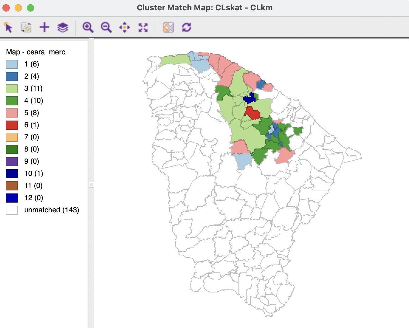
Figure 12.10: Cluster Match Map - SKATER and K-MEANS

In sum, rather than having to rely on a visual assessment of the overlap between clusters, the Cluster Match Map provides a simple numeric summary.