9.2 Clustering on Geographic Coordinates
Applying classic cluster methods to geographical coordinates results in clusters as regions in space. There is nothing special to this type of application. In fact, a number of examples of this approach have already been illustrated in previous chapters.
When using actual geographical coordinates as the features in a clustering exercise, it is important to make sure that the Transformation is set to Raw. This is to avoid distortions in the distance measure that may result from the transformations, such as z-standardize.
For example, in cases where one dimension dominates the other, the range of the coordinates in one direction (e.g., North-South) can be much greater than the range in the other direction (East-West). Standardization of the coordinates would result in the transformed values to be more compressed in the dominant direction, since both transformed coordinates end up with the same variance. This will directly affect the resulting inter-point distances used in the dissimilarity matrix.
In addition, it is critical that the geographical coordinates are projected and not simply latitude-longitude decimal degrees. This ensures that the Euclidean distances are calculated correctly. Using latitude and longitude to calculate straight line distance is incorrect.
For most methods, the clusters will tend to result in fairly compact regions. For example, for K-Means, the regions correspond to Thiessen polygons around the cluster centers. K-Medoids are the solution to a form of location-allocation problem, with the cluster center serving as the location and the cluster members containing the allocation or service area. For spectral clustering, the boundaries between regions can be more irregular. Finally, for hierarchical clustering, the result depends greatly on the linkage method chosen. In most situations, Ward’s and complete linkage will yield the most compact regions. In contrast, single and average linkage will tend to result in singletons and/or long chains of points.
9.2.1 Implementation
The cluster methods are invoked in the standard manner, as illustrated in Chapters 5 to 8. The only difference is in the selection of variables.
If included among the data set variables, X and Y coordinates can be selected in the same way as any other variable. This is quite flexible, and allows any pair of variables to be chosen as coordinates, although to some extent, that defeats the purpose.
An alternative is to select the coordinates as <X-Centroids> and <Y-Centroids> (at the bottom of the variables list in the Clustering Settings dialog), as in Section 7.3.3. This selection invokes a check on the proper projection (a warning will be generated for latitude-longitude decimal degrees). As mentioned, the Transformation is best set to Raw to keep the original dimensions.
The corresponding cluster maps are shown in Figures 9.1 and 9.2, respectively for K-Means and K-Medoids, and for Spectral and Hierarchical clustering. The number of clusters is set to 12. In each instance, the defaults were used, with knn=8 for Spectral Clustering and Ward’s linkage for Hierarchical Clustering.44 The clusters vary slightly in fit, with K-Means obtaining the highest BSS/TSS ratio at 0.941, followed closely by Hierarchical Clustering (0.937) and K-Medoids (0.933). Spectral Clustering does slightly less well at 0.929. Overall, however, these results reveal excellent cluster separation.
Nevertheless, the corresponding spatial patterns are quite distinct. The largest clusters range from 34 observations for Hierarchical Clustering to 20 for Spectral Clustering. For all but K-Medoids, the location of the largest cluster is in the North-East of the state, but for K-Medoids, it is at the South-Eastern tip of the state. The spatial layout is similar in broad strokes, with most clusters fairly compact and aligning with the state border. One to two clusters make up the central regions. However, there are many differences as well. This illustrates that even when only spatial considerations are taken into account, the respective methods result in varying layouts.
More formal comparisons of the spatial features of clusters are considered in Chapter 12.
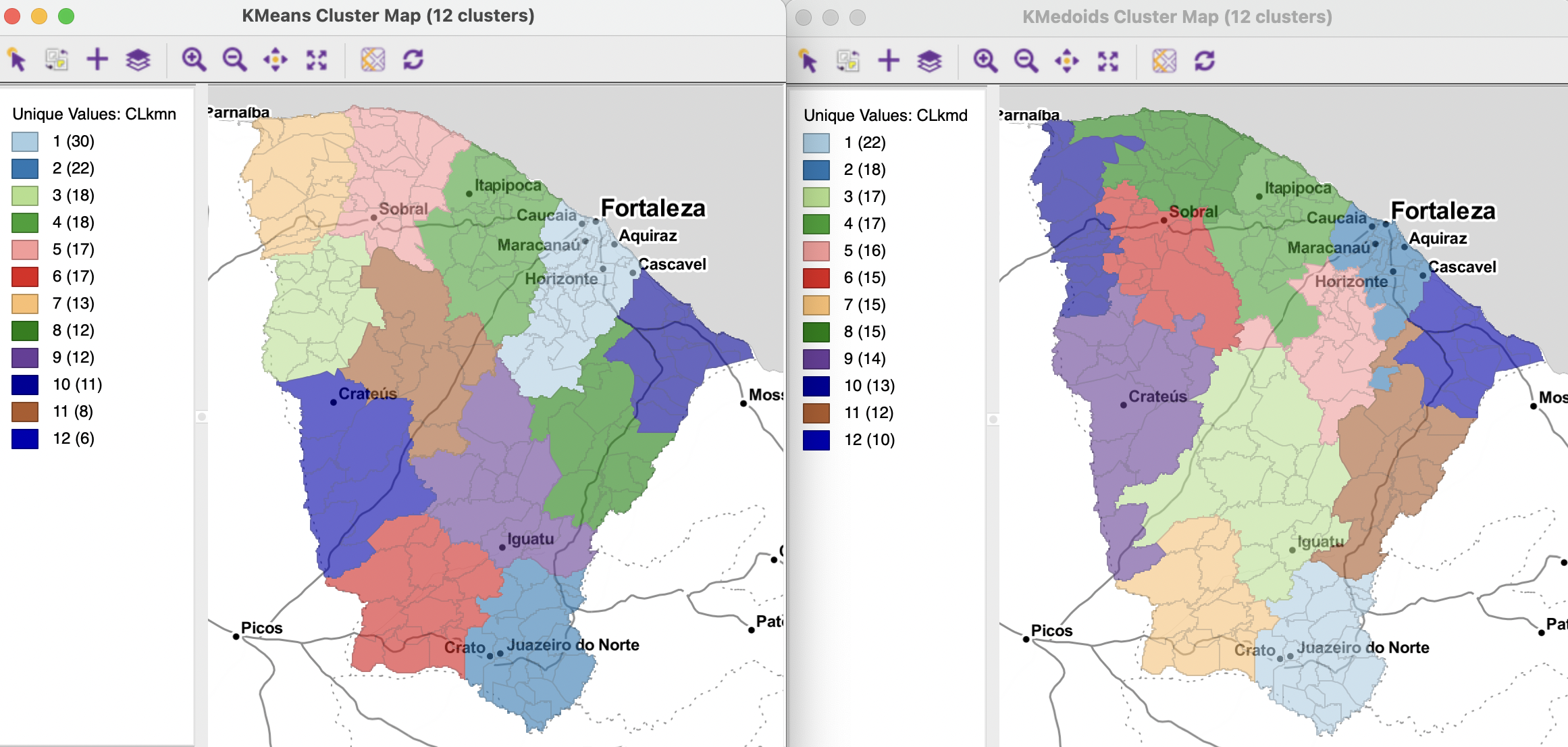
Figure 9.1: K-Means and K-Medoids on X-Y Coordinates
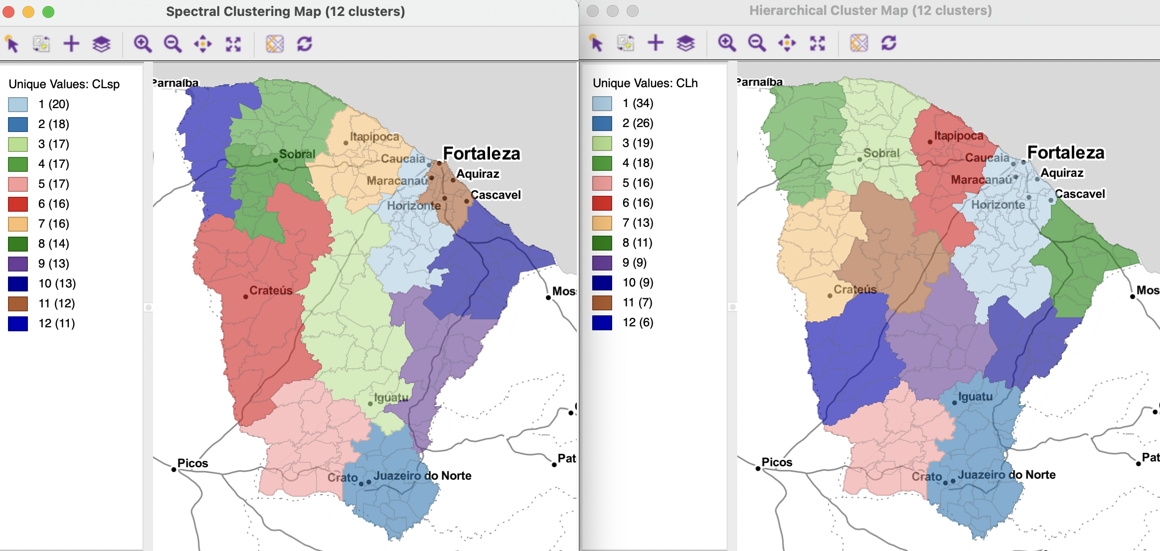
Figure 9.2: Spectral and Hierarchical on X-Y Coordinates
The maps are shown with a Stamen > Toner Lite base layer in order to situate the clusters in context.↩︎