4.4 Implementation
The t-SNE functionality is invoked from the drop down list created by the toolbar Clusters icon (Figure 4.1), as the third item (more precisely, the third item in the dimension reduction category). Alternatively, from the main menu, Clusters > t-SNE gets the process started.
To illustrate these methods, the same ten bank indicators are used as in the previous chapter (for a full list, see Section 3.2.2).
The main dialog is the t-SNE Settings panel, shown in Figure 4.2. The left-hand side contains the list of available variables as well as several parameters that can be specified to fine tune the algorithm. Both Euclidean and Manhattan distance metrics are available for the Distance Function (to compute the probability functions), with Euclidean as the default. As before, the Standardize (Z) is the default Transformation.
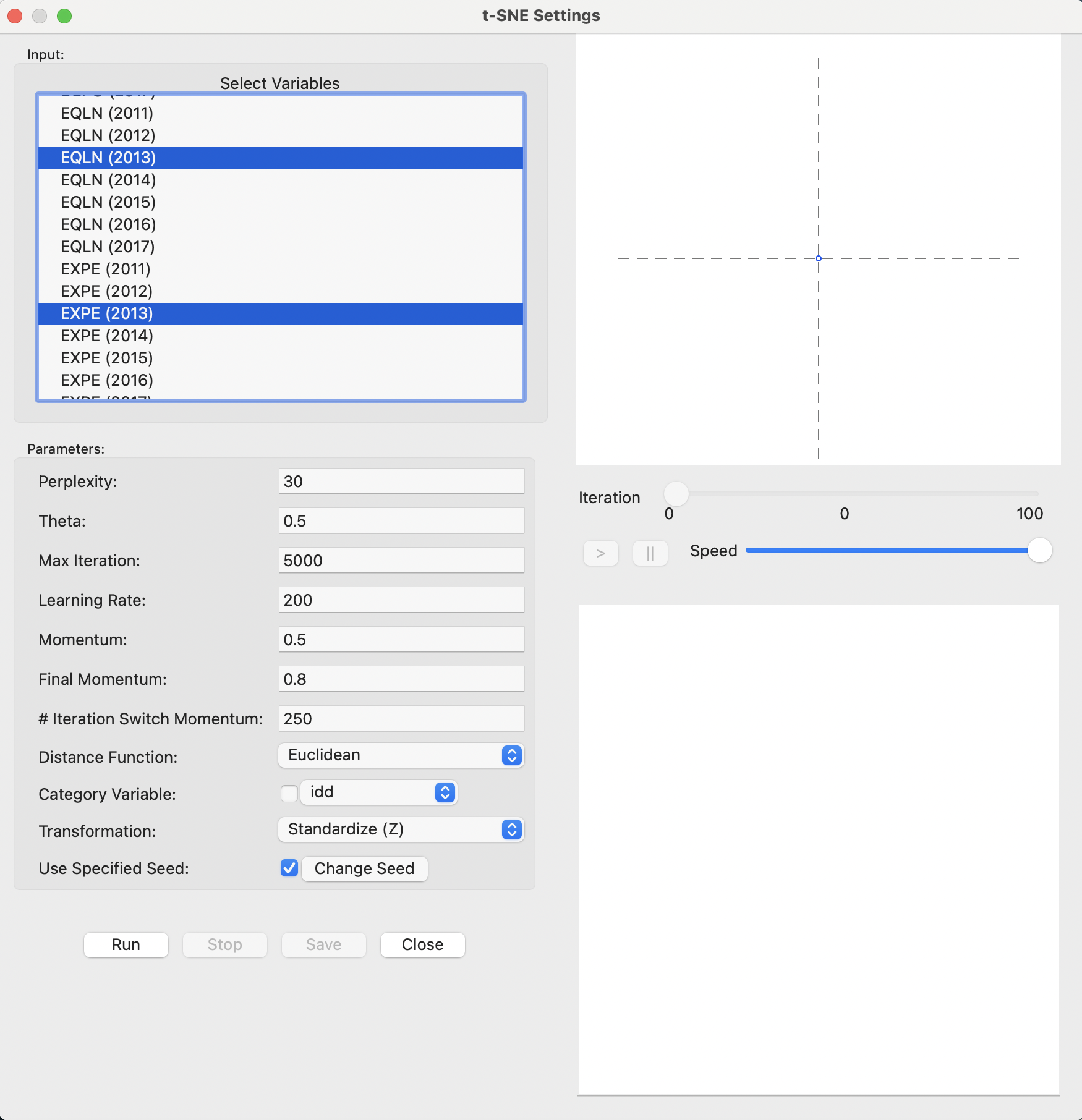
Figure 4.2: t-SNE Settings
On the right-hand side of the interface are two major panels. The top consists of a space that is used to track the changes in the two-dimensional scatter plot as the iterations proceed. The bottom panel gives further quantitative information on the evolution of the quality of the result, reported for every 50 iterations. This lists a value for the error, i.e., the cost function evaluated at that stage. The table provides an indication of how the process is converging to a stable state.
In-between the two result panes on the right is a small control panel to adjust the speed of the animation, as well as allowing to pause and resume as the iterations proceed (see Section 4.4.1).
With all the parameters left to their default settings, the Run button populates the panels on the right-hand side. Figure 4.3 shows the result after the default 5000 iterations, with a final cost of 0.714386. The top panel contains the familiar scatter plot of the t-SNE coordinates in two dimensions. The bottom pane (only partly shown) lists the final cost as well as the error for every 50 iterations. It shows that the error has been hovering around a similar value for (at least) the last 500 iterations.
In the implementation in GeoDa, the final cost value listed (0.714386) does not exactly equal the result for the error at the last iteration (0.713598). This is due to the use of the Barnes-Hut approximation (Section 4.3.2.2).19
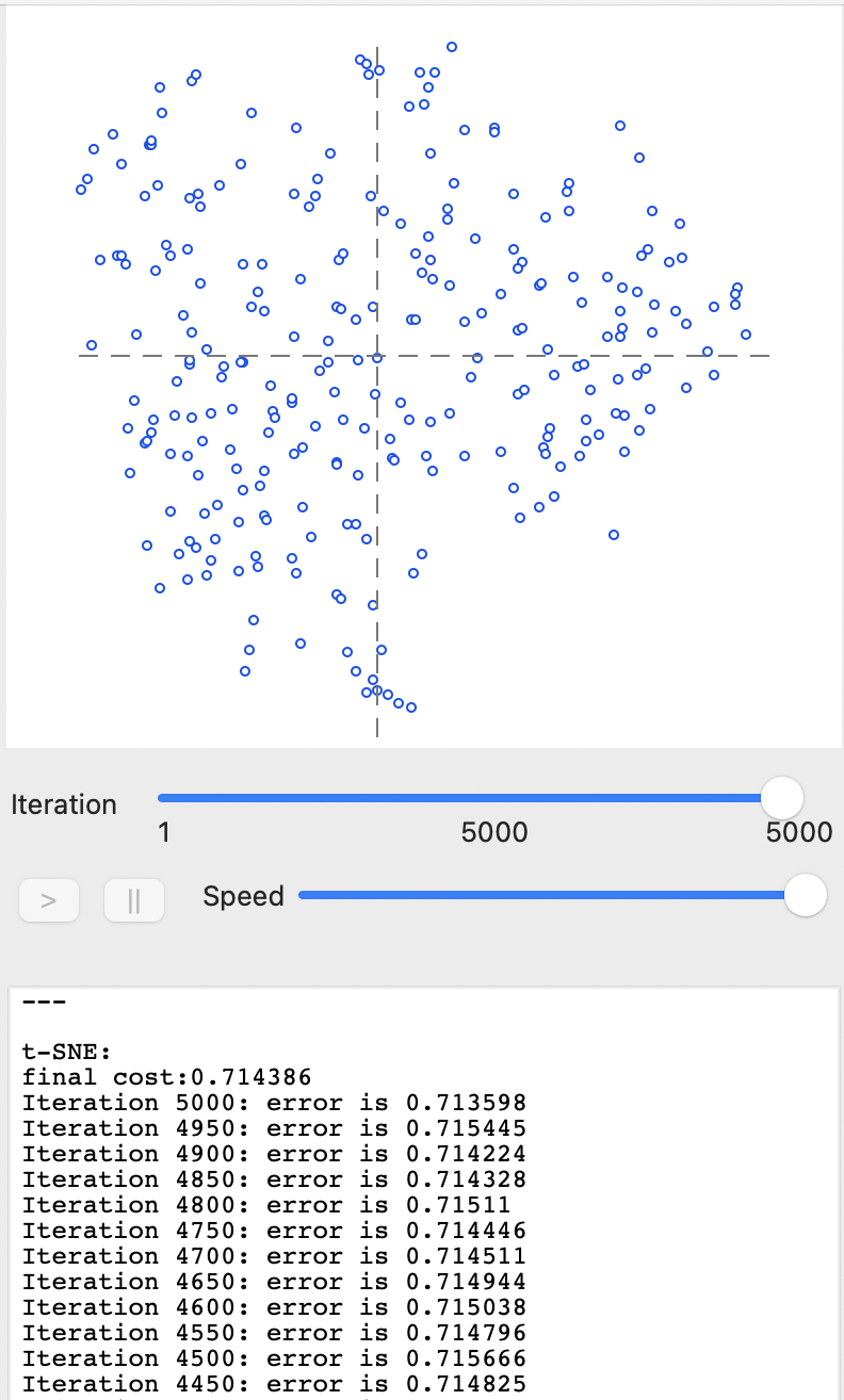
Figure 4.3: t-SNE after full iteration - default settings
With the final result in hand, selecting the Save button brings up the familiar dialog to specify the variable names to be saved to the data table (defaults are V1 and V2, but here set to V1tsne and V2tsne). Once these coordinate variables are specified, the final scatter plot is generated in a separate window, as illustrated in Figure 4.4.
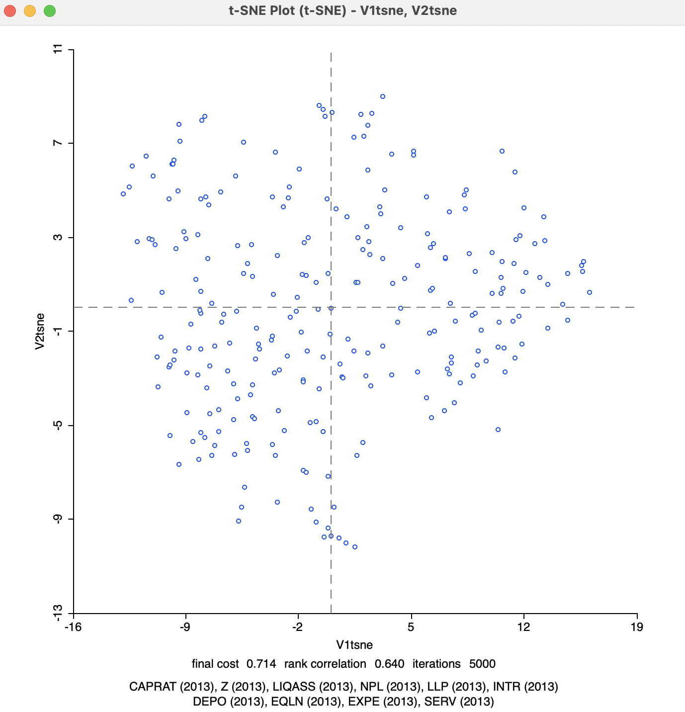
Figure 4.4: t-SNE 2D Coordinates
At the bottom of the graph is a listing of the variables used in the analysis, as well as the final cost (0.714), the rank correlation (0.640), and the number of iterations (the default 5000). Since the t-SNE optimization algorithm is not based on a specific stopping criterion, unless the process is somehow paused (see Section 4.4.1), the number of iterations will always correspond to what is specified in the options panel. However, this does not mean that it necessarily has resulted in a stable optimum. In practice, one therefore needs to pay close attention to the point pattern of the iterations as they proceed.
The final cost is not comparable to the objective function for MDS, since it is not based on a stress function. On the other hand, the rank correlation is a rough global measure of the correspondence between the relative distances and remains a valid measure. However, it should be kept in mind that t-SNE is geared to optimize local distances, so a global performance measure is not necessarily the best measure of performance.
4.4.0.1 Inspecting the iterations
The bottom panel allows for an inspection of the results for the error at each iteration. A more visual representation of the change in point configurations can be found by manipulating the Iteration button in the top panel. As the button is moved to the left, the change in configuration is illustrated in the graph as the optimization process proceeds.
This is particularly illuminating in the beginning stages of the algorithm, where substantial jumps can be observed. For example, in Figure 4.5, the Iteration is shown for two early results, one at iteration 250 (error 54.7166) and one shortly afterwards, at iteration 300 (error 0.852884). This is the point in the solution process where initial very chaotic solutions (jumping from one side of the graph to the other) begin to stabilize to a more circular cloud shape.
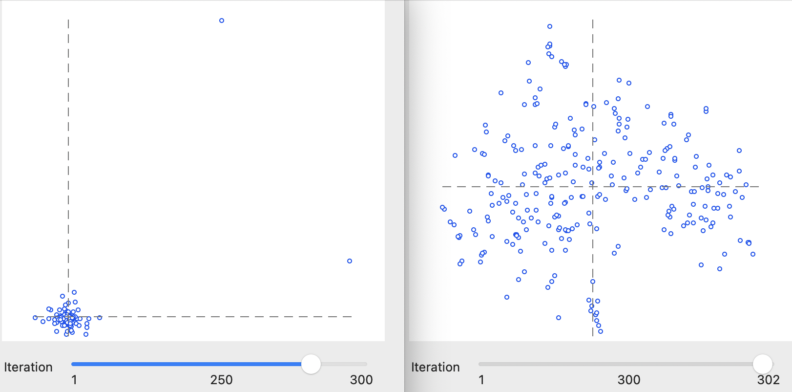
Figure 4.5: Inspecting interations of t-SNE algorithm: 250 and 300
This process continues until a certain degree of stability is obtained, after which the changes become marginal. For example, in Figure 4.6, the results at 2500 iterations (error 0.71491) and at 4000 iterations (error 0.715028) are shown, which portray a very similar pattern with almost identical error measures, near impossible to distinguish from the final solution in Figure 4.3.
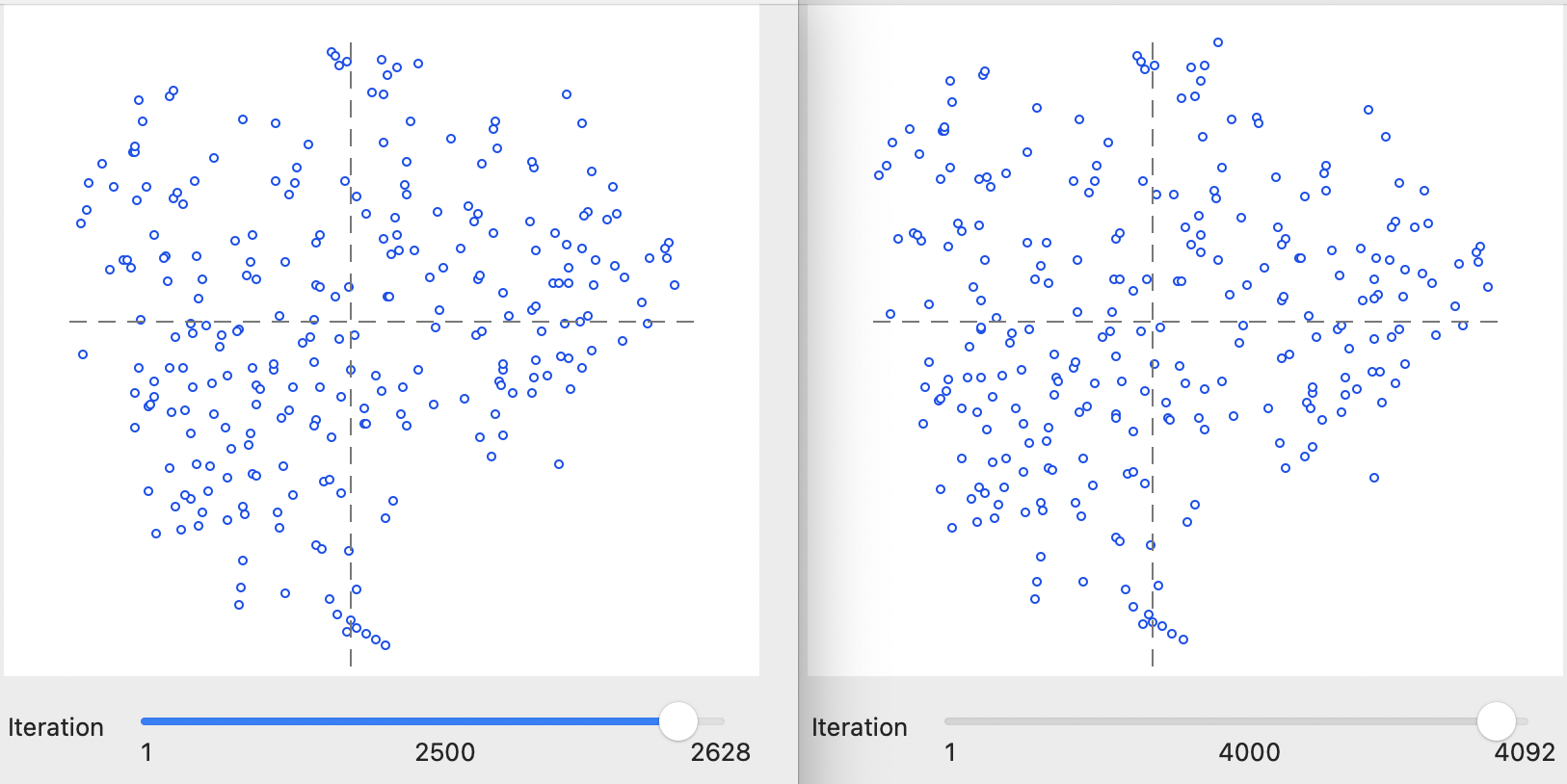
Figure 4.6: Inspecting interations of t-SNE algorithm: 1000 and 3000
4.4.1 Animation
As mentioned, with the default settings, the optimization runs its full course for the number of iterations specified in the options. The Speed button below the graph on the right-hand side allows for the process to be slowed down for visualization purposes, by moving the button to the left. This provides a very detailed view of the way the optimization proceeds, gets trapped in local optima and then manages to move out of them.
In addition, the pause button (||) can temporarily halt the process. The resume button (>) continues the optimization. The iteration count is given below the graph and in the bottom panel the progression of the cost minimization can be followed.
In this implementation, the pause button is different from the Stop button that is situated below the options in the left-hand panel. The latter ends the iterations and freezes the result, without the option to resume. However once frozen, one can move back through the previous sequence of iterations by moving the Iteration button to the left.
4.4.2 Tuning the Optimization
The number of options to tune the optimization algorithm may seem a bit overwhelming. However, in many instances, the default settings will be fine, although some experimenting is always a good idea.
To illustrate the effect of some of the options, changes in three central parameters are illustrated in turn: Theta, Perplexity, and the Iteration Switch for the Momentum.
4.4.2.1 Theta
The Barnes-Hut algorithm implemented for t-SNE sets the Theta (\(\theta\)) parameter to 0.5 by default. This is the criterion that determines the extent of simplification for the \(q_{ij}\) measures in the gradient equation. The parameter is primarily intended to allow the algorithm to scale up to large data sets.
In smaller data sets, like in the example considered here, this may be set to zero, which can speed up the solution since the actual distances are used, rather than a proxy. The result is shown in Figure 4.7. The final cost is 0.737581 with a rank correlation of 0.635, both slightly worse than the default. In this case, convergence is reached after fewer than 1000 iterations, somewhat faster than for the default case. Also, in this instance, there is no difference between the error at the last iteration and the final cost, since no Barnes-Hut simplification is carried out.
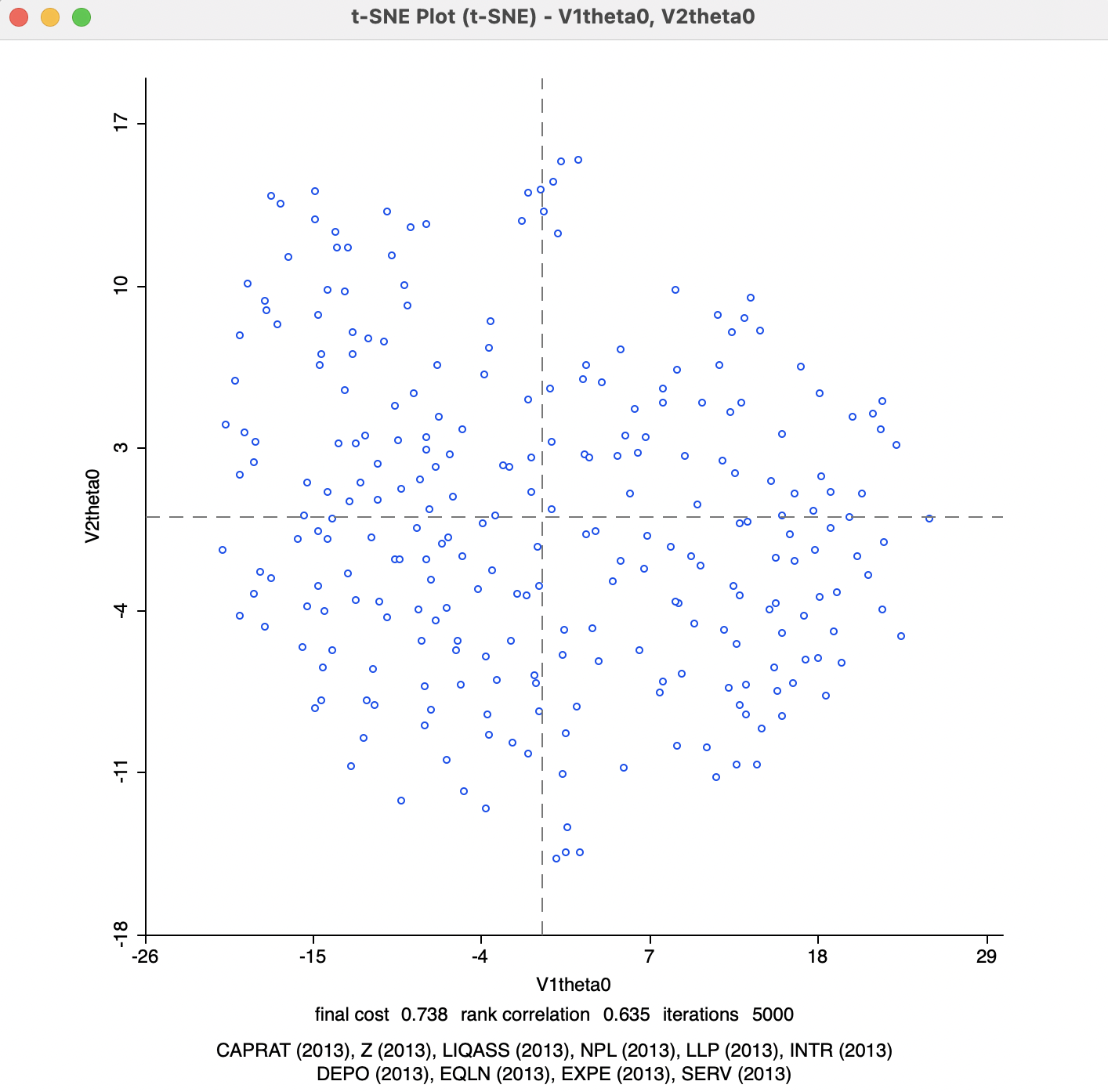
Figure 4.7: t-SNE 2D Coordinates for theta=0
4.4.2.2 Perplexity
The second parameter to adjust is the Perplexity (with Theta set back to its default value). This is a rough proxy for the number of neighbors and is by default set to a value of 30. The results for a value of 50 (the highest suggested by van der Maaten and Hinton 2008) are visualized in Figure 4.8. Compared to the previous results, the cost is much lower at 0.540604, and a higher rank correlation of 0.689. Convergence is reached after about 1600 iterations.
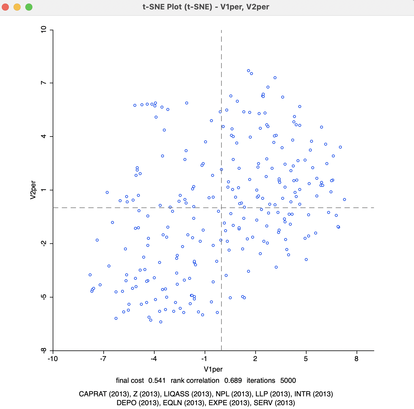
Figure 4.8: t-SNE 2D Coordinates for perplexity=50
4.4.2.3 Iteration momentum switch
The final adjustment is to the Iteration Switch for the Momentum parameter, which decides at which point in the iterations the Momentum moves from 0.5 to 0.8. The default value is 250. With Perplexity left at 50, a change of the Iteration Switch to 100 obtains less chaotic solutions much sooner than in the previous cases. The switch happens between 100 and 150 iterations. The end result, shown in Figure 4.9, is the best achieved so far: the final cost is 0.525096 with a rank correlation of 0.700.
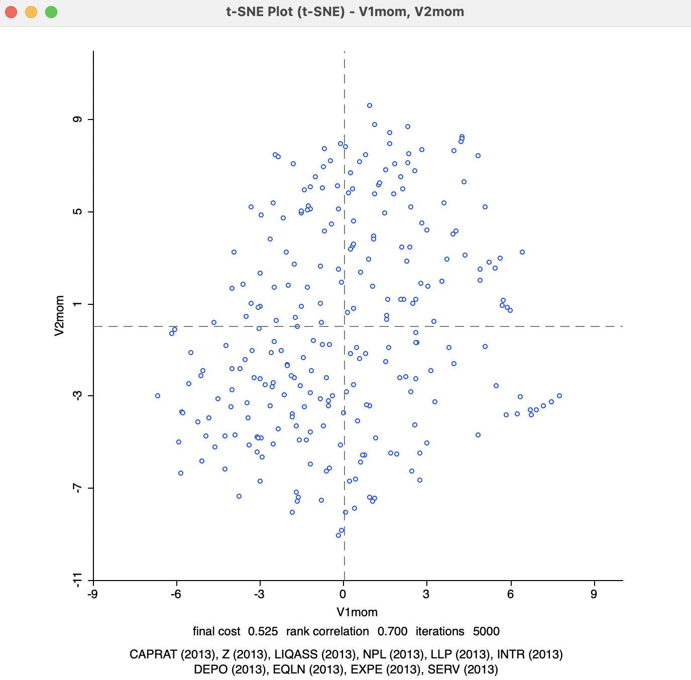
Figure 4.9: t-SNE 2D Coordinates for perplexity=50, momentum=100
Further experimentation with the various parameters can provide deep insight into the dynamics of this complex algorithm, although the specifics will vary from case to case. Also, as argued in van der Maaten (2014), the default settings are an excellent starting point.
4.4.3 Interpretation and Spatialization
All the visualization options reviewed for classic MDS in Chapter 3 can be applied to the t-SNE solutions, in the same way as described in Sections 3.4 and 3.5. This includes the incorporation of a categorical variable that is visualized in the coordinate plot (see Section 3.4.2). In addition, for t-SNE, those categories are also shown during the iterations and animations in the top right panel of Figure 4.2. Otherwise, everything operates as discussed previously.
One aspect that remains to be investigated is the extent to which the t-SNE approach yields solutions that provide a match with geographic neighbors. This would be reflected in a nearest neighbor match test based on t-SNE nearest neighbors.
4.4.3.1 Nearest neighbor match test
The nearest neighbor match test is illustrated for the coordinates of the latest t-SNE results, V1mom and V2mom. The k-nearest neighbors with k=6 are matched to the geographical k-nearest neighbors. The corresponding unique values cardinality map is depicted in Figure 4.10. Compared to the MDS results in Figure 3.17 and the standard results in Figure 3.18, the largest number of common neighbors is four, obtained for one observation (the Cassa Raiffeisen in Latsch in the Trentino-Alto Adige Region, observation 67). The associated probability is 0.000001, suggesting very strong evidence of a multivariate local cluster. In addition, there are 6 observations with three common neighbors (p=0.000133), and 23 with two common neighbors (p=0.006275). As shown in Section 3.5.3, the result with one common neighbor cannot be deemed to be significant (p=0.125506).
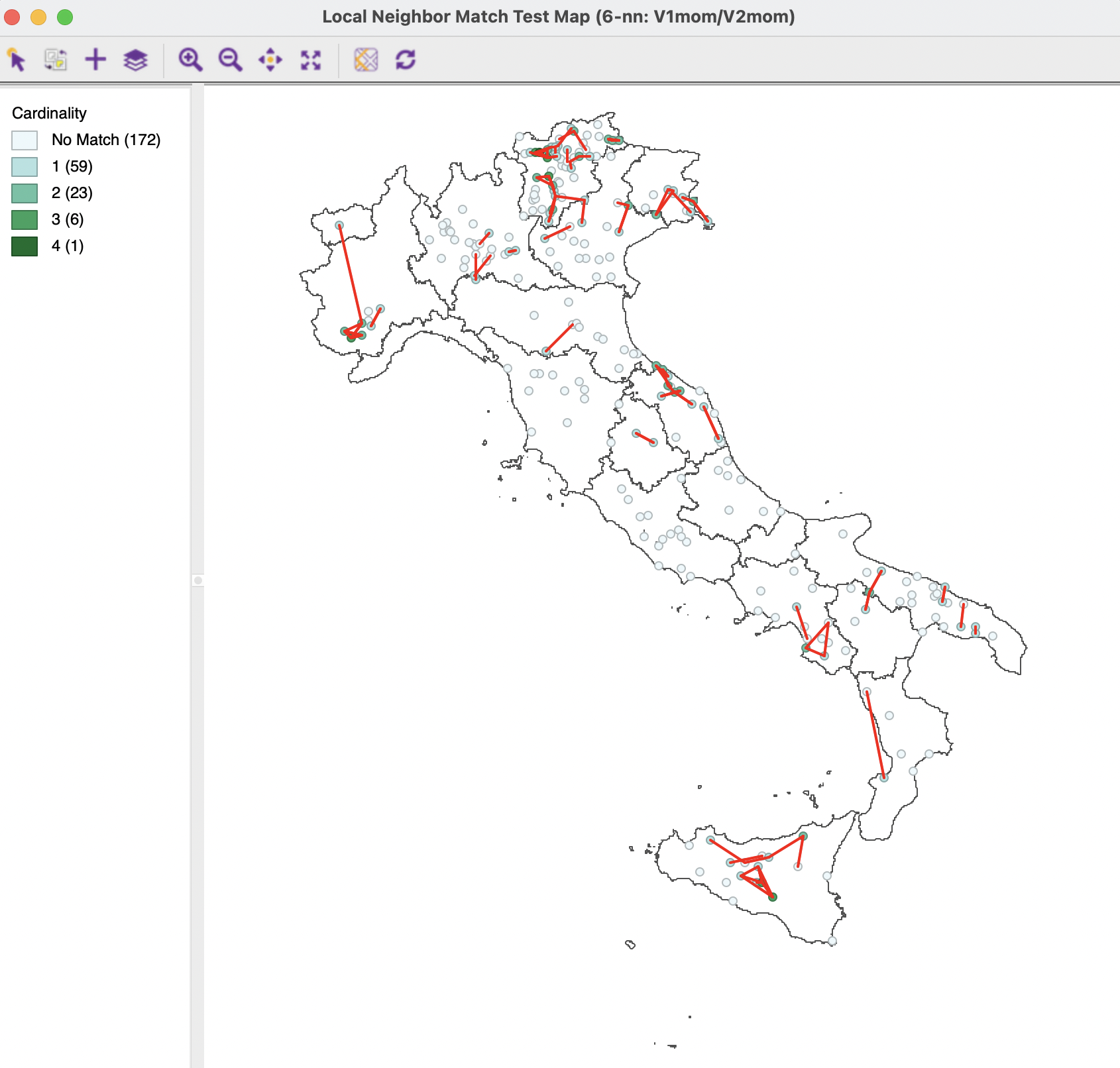
Figure 4.10: Nearest Neighbor Match Test for t-SNE
The cluster analysis based on the t-SNE computations yields the most significant clusters in the current example. This is somewhat to be expected, since the method stresses local similarities between the higher and lower embedded dimension. Many identified locations match the standard cluster results, but several are also in different locations. The involved trade offs remain to be further investigated.
As detailed in Section 4.3.2.2, when Theta is not zero, several values of \(q_{ij}\) are replaced by the center of the corresponding quadtree block. The final cost reported is computed with the values for all \(i-j\) pairs included in the calculation, and does not use the simplified \(q_{ij}\), whereas the error reported for each iteration uses the simplified version.↩︎