2.5 Spatializing Principal Components
A distinct perspective towards principal component analysis is taken by spatializing the visualization, i.e., by directly connecting the value for a principal component to its geographical location. As pointed out before, care must be taken in interpreting the results, since the sign for the component may depend on the method used to compute it. Two special forms of visualization are considered.
One is a thematic map, which may suggest patterns in the values obtained for the components. Mapping of principal components was pioneered in botany and numerical ecology, going back as far as an early paper by Goodall (1954), where principal component scores were mapped using contour lines. A recent review is given in Dray and Jombart (2011).
Dray and Jombart (2011) also consider the global spatial autocorrelation among individual principal components, specifically Moran’s I, as well as the principal components associated with its extension to multivariate analysis (Dray, Saïd, and Débias 2008).7 However, they do not consider local indicators of spatial autocorrelation. The application of those local cluster methods to principal components provides a univariate alternative to the multivariate cluster analysis considered in Chapter 18 of Volume 2.
2.5.1 Principal component map
Figure 2.12 illustrates the caution needed when interpreting a map of principal component values. In the left-hand panel, a box map is shown of the second principal component obtained through the SVD method, PC2. On the right is a box map of the same component, but now computed using the Eigen method, PC2e. Clearly, what is high on the left, is low on the right. Specifically, the two upper outliers on the left (observations in the red rectangle) become two lower outliers on the right (observations in the blue rectangle). As a result, what is high or low is less important than the notion of multivariate similarity. Observations in the same category share a multivariate similarity that is summarized in the principal component.
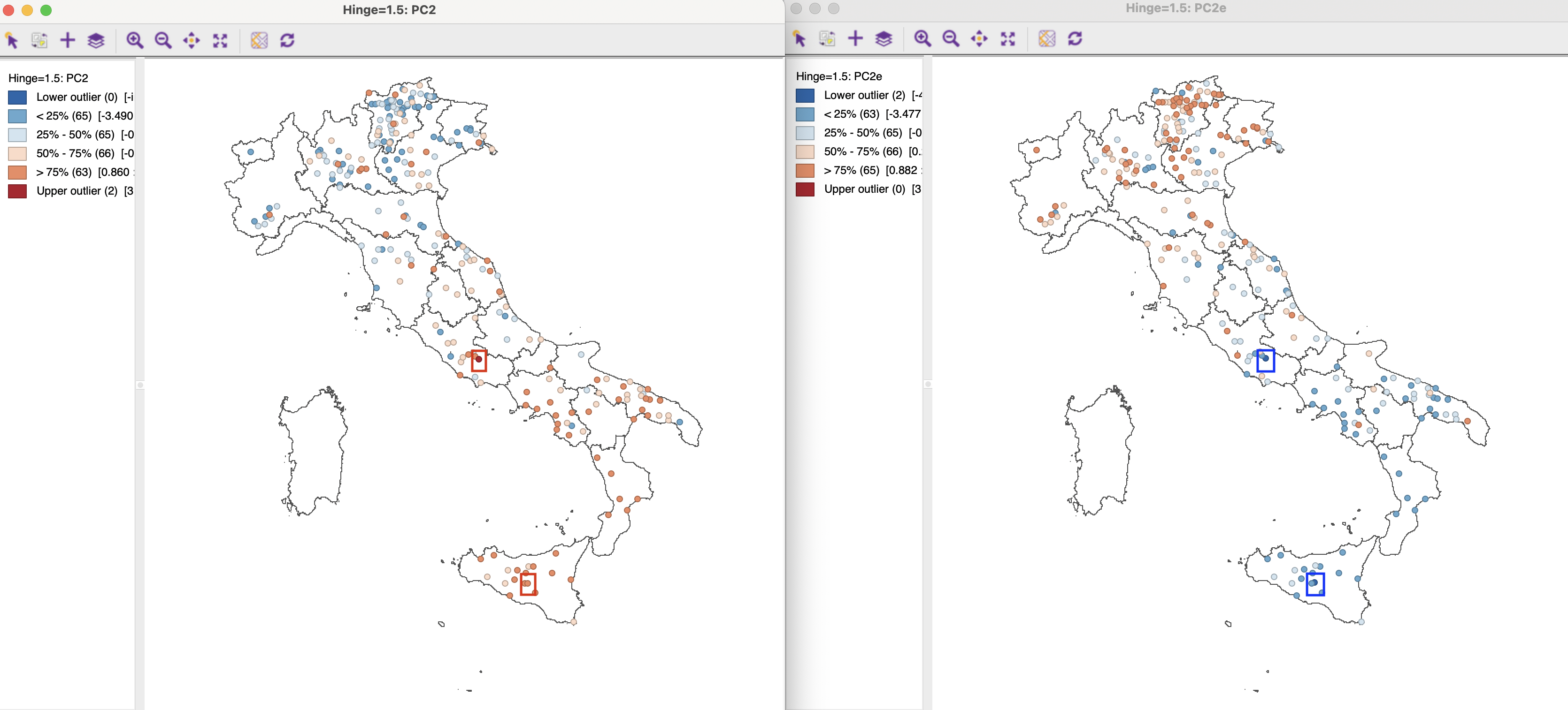
Figure 2.12: Box Map of Second Principal Component
2.5.2 Univariate cluster map
A principal component can be treated as any other variable in a local cluster analysis. For example, in the left-hand panel of Figure 2.13, the 19 observations identified as the cores of Low-Low clusters are selected, based on the Local Geary statistic, using queen contiguity for the point locations, 99,999 permutations and p < 0.01.8 The matching observations in the parallel coordinate plot on the right illustrate a clustering along multivariate dimensions.
The univariate local cluster map for a principal component can thus be used as a proxy for multivariate clustering of the variables that are the main contributors to the component.
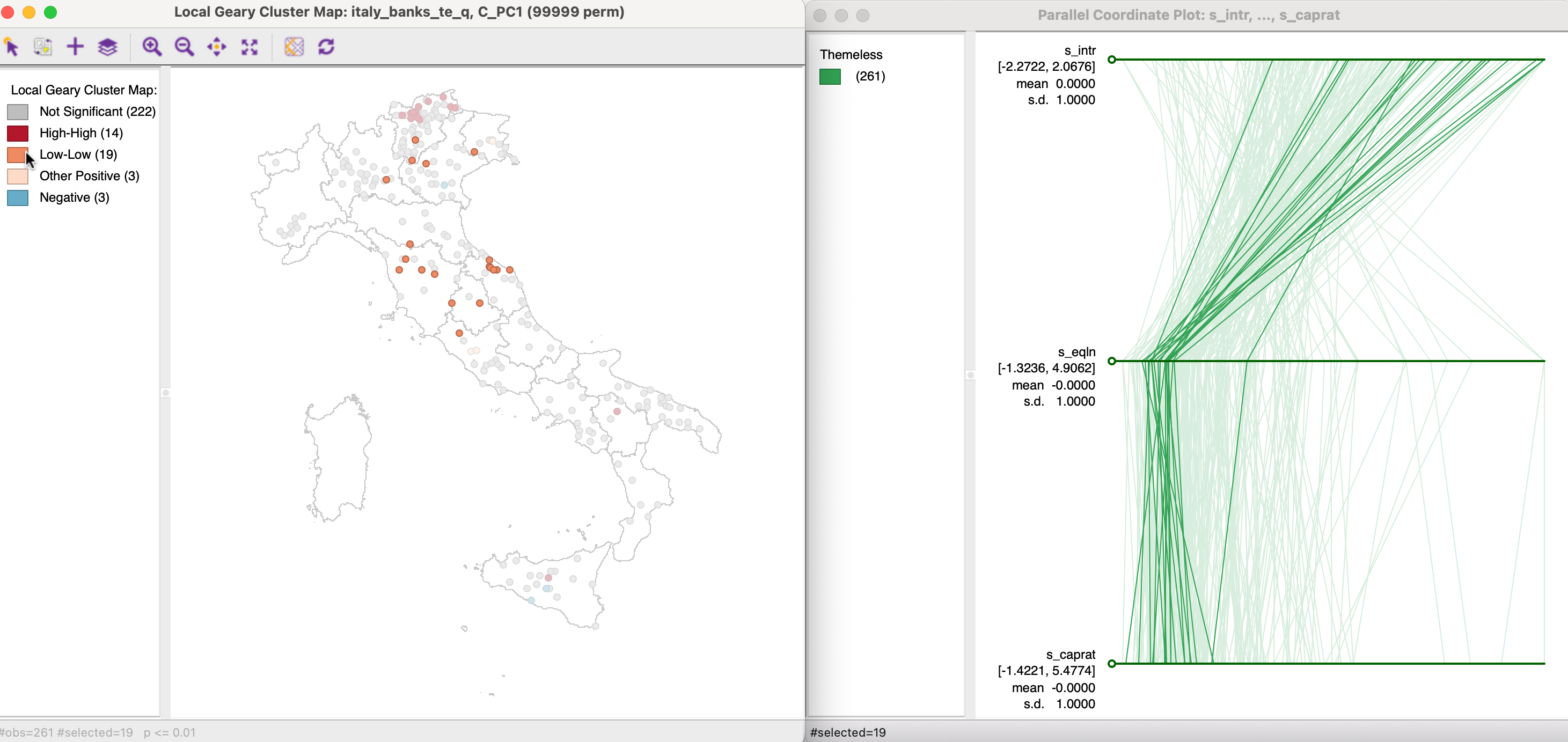
Figure 2.13: Principal Component Local Geary Cluster Map and PCP
2.5.3 Principal components as multivariate cluster maps
An even closer look at the correspondence between univariate clustering for a principal component and its multivariate counterpart is offered by Figure 2.14. On the left is the same Local Geary cluster map as in Figure 2.13, but now linked to a multivariate Local Geary cluster map for the three main contributing variables (s_intr, s_eqln, and s_caprat). The latter is also based on queen contiguity, with 99,999 permutations and p < 0.01. The total number of significant locations in both maps is very similar: 39 in the univariate map and 43 in the multivariate map. Interestingly, the number of spatial outliers is almost identical, with two of them identified for the same locations on the island of Sicily, highlighted by the blue rectangle.
There is also close correspondence between several cluster locations. For example, the High-High cluster in the north-east Trentino region and the Low-Low cluster in the region of Marche are shared by both maps (highlighted within a green rectangle). While these maps may give similar impressions, it should be noted that in the multivariate Local Geary each variable receives the same weight, whereas the principal component is based on different contributions by each variable.
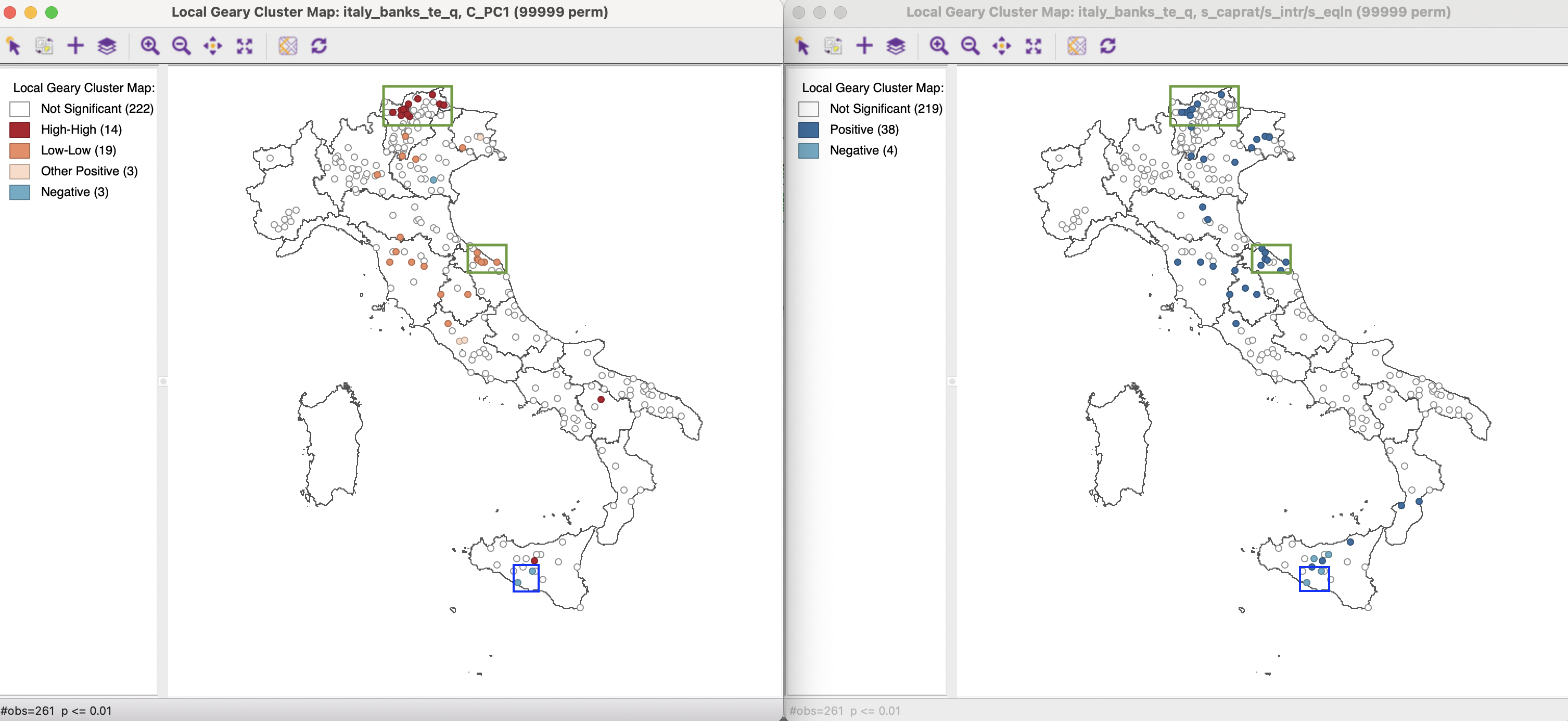
Figure 2.14: Principal Component and Multivariate Local Geary Cluster Map
These findings again suggest that in some instances, a local spatial autocorrelation analysis for one or a few dominant principal components may provide a viable alternative to a full-fledged multivariate analysis. This constitutes a spatial aspect of principal components analysis that is absent in standard treatments of the method.