11.3 Max-P Region Problem
The max-p region problem, outlined in Duque, Anselin, and Rey (2012), makes the number of regions (\(p\)) part of the solution process. This is accomplished by introducing a minimum size constraint for each cluster. In contrast to the use of such a constraint in earlier methods, where this was optional (see, for example, Section 10.3.2.2), for max-p the constraint is required. The size constraint is either a minimum value for a spatially extensive variable (such as population size, number of housing units), or a minimum number of spatial units that need to be contained in each region. Initially formulated as a standard regionalization problem, the method was extended to take into account the compactness of the solutions in Feng, Rey, and Wei (2022), as well as applied to a network structure in She, Duque, and Ye (2017).
In Duque, Anselin, and Rey (2012), the solution to the max-p region problem was presented as a special case of mixed integer programming (MIP), building on earlier approaches to incorporate contiguity constraints in site design problems given by Cova and Church (2000). Two key aspects are the formal incorporation of the contiguity constraint and the use of an objective function that combines the number of regions (\(p\)) and the overall homogeneity (minimizing the total with sum of squares). However, within this objective function, priority is given to finding a larger \(p\) rather than the maximum homogeneity. In contrast to an unconstrained problem, where a larger \(p\) will always yield a better measure of homogeneity (see the discussion of the elbow graph for K-means clustering in Section 6.3.4.2), this is not the case when both a minimum size constraint and contiguity are imposed. In other words, simple minimization of the total within sum of squares may not necessarily yield the maximum \(p\). Also, the maximum \(p\) solution may not give the best total within sum of squares. The trade off between the two sub-objectives is made explicit.
In a nutshell, the max-p algorithm will find the largest \(p\) that accommodates both the minimum size and contiguity constraints and then finds the regionalization that yields the smallest total within sum of squares.
As it turns out, the formal MIP strategy becomes impractical for any but small size problems. Instead, a heuristic was proposed that consists of three important steps: growth, assignment of enclaves, and spatial search.54 As was the case for previous heuristics, this does not guarantee that a global optimum is found. Therefore, some experimentation with the various solution parameters is recommended. Even more than in the case of AZP, sensitivity analysis and the tuning of parameters is critical to find better solutions. Simply running the default will not be sufficient. The trade offs involved are complex and not always intuitive.
11.3.1 Max-p Heuristic
The max-p heuristic outlined in Duque, Anselin, and Rey (2012) consists of three important phases: growth, assignment of enclaves, and spatial search.
The objective of the first phase is to find the largest possible value of \(p\) that accommodates both the minimum bounds and the contiguity constraints. In order to accomplish this, many different spatial layouts are grown by taking a random starting point and adding neighbors (and neighbors of neighbors) until the minimum bound is met. While it is practically impossible to consider all potential layouts, repeating this process for a large number of tries with different starting points will tend to yield a high value for \(p\) (if not the highest), given the constraints.
In the process of growing the layout, some spatial units will not be allocated to a region, when they and/or their neighbors do not meet the minimum bounds constraint or break the contiguity requirement. Such spatial units are stored in an enclave.
At the end of the growth process, the result consists of one or more spatial layouts with \(p\) regions, where \(p\) is the largest value that could be obtained. Before proceeding with the optimization process, any remaining spatial units that are contained in the enclave must be assigned to an existing region. This is implemented in such a way that the overall within sum of squares is minimized.
Once all units have been assigned to one of the \(p\) regions, the best solution is selected as the initial feasible solution. At this point, the heuristic proceeds in exactly the same way as for AZP, using either greedy search, tabu search, or simulated annealing to find a (local) optimum. The best overall solution is chosen at the end.
11.3.1.1 Illustration
To continue the illustration of the heuristic by means of the Arizona county example, the population in 1990 (PO90) is added as the minimum size constraint. Specifically, a lower limit of a population size of 250,000 is imposed (without any substantive meaning, purely to illustrate the logic of the algorithm). In Figure 11.15, the population count is shown for each county. The other variables are as before (see Section 10.2.1).
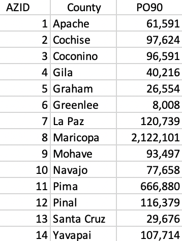
Figure 11.15: Arizona counties population
The heuristic consists of three phases. In the first, the growth phase, feasible regions are created and the largest possible \(p\) identified. For those configurations that achieve the maximum \(p\), any unassigned spatial units, the so-called enclave, are allocated to existing regions so as to minimize the total within sum of squares. Finally, the best of these solutions is taken as a feasible initial solution to start the optimization process. The latter is the same as for AZP.
The growth process is initiated by randomly selecting a location and determining its neighbors. In Figure 11.16, county 6 is chosen. Its three neighbors are 1, 5 and 2.
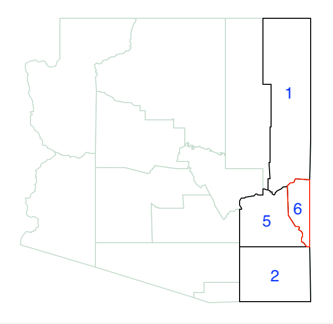
Figure 11.16: Arizona max-p growth, start with 6
County 6 has a population of 8,008. Its neighbor with the largest population is county 2, with a population of 97,624. Joined with 6 it forms the core of the first region. Its total population is now 105,632, which does not meet the minimum threshold. At this point, the neighbors of 2 that are not already neighbors of 6 are added to the neighbor list.
As shown in Figure 11.17, the neighbor set now also includes 11 and 13.
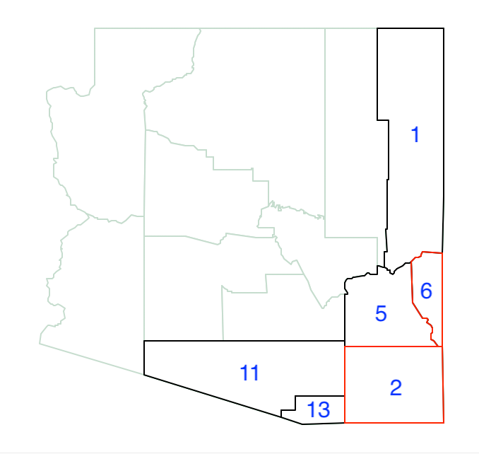
Figure 11.17: Arizona max-p growth phase - 6 and 2
Of the four neighbors, county 11 has the largest population (666,880), which brings the total regional population to 764,504, well above the minimum bound. At this point, the first region becomes 6-2-11, shown in Figure 11.18.
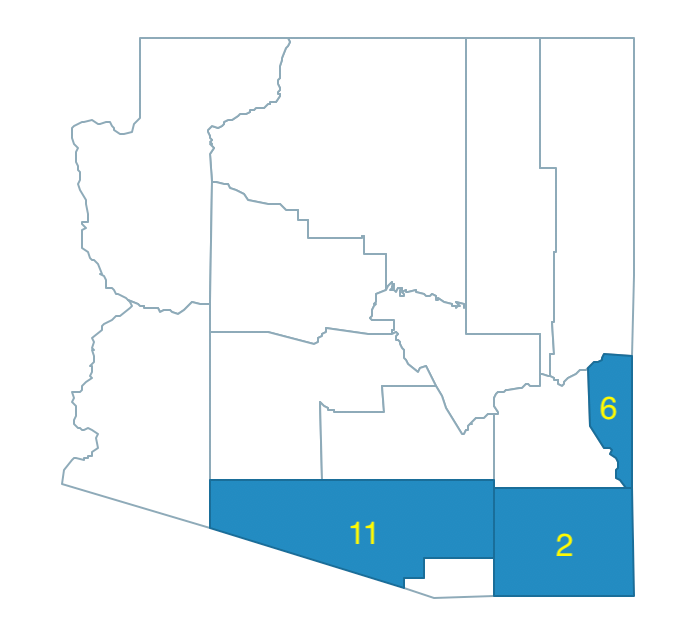
Figure 11.18: Arizona max-p growth phase - region 1
The second random seed yields county 8. Its population is 2,122,101, well above the minimum bound. Therefore, it constitutes the second region in the growth process as a singleton, shown in Figure 11.19.
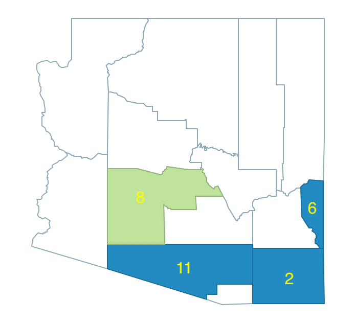
Figure 11.19: Arizona max-p growth phase - regions 1 and 2
The third random seed is county 3, with neighbors 9, 14, 4 and 10, shown in Figure 11.20. The population of county 3 is 96,591 and the largest neighbor is 14, with a population of 107,714. This yields a total of 204,305, insufficient to meet the minimum bound.
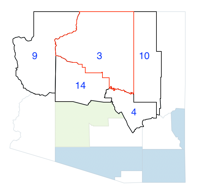
Figure 11.20: Arizona max-p growth phase - pick 3
Therefore, again counties 3 and 14 are grouped and the list of neighbors updated, shown in Figure 11.21. The only new neighbor is county 7, since county 8 has already been allocated to the second region.
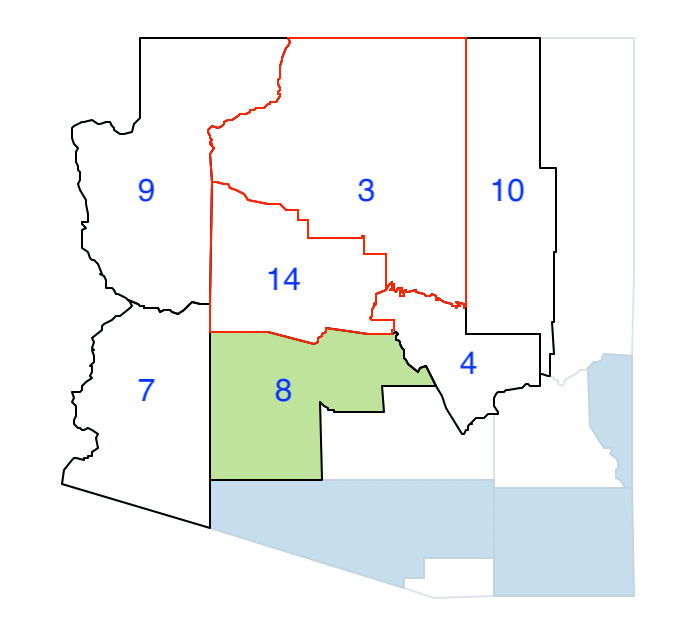
Figure 11.21: Arizona max-p growth phase - join 3 and 14
Since county 7 has the largest population among the eligible neighbors (120,739) it is grouped with counties 3 and 14. This new region meets the minimum threshold, with a total population of 325,044. At this point, there are three regions (\(p = 3\)), shown in Figure 11.22.
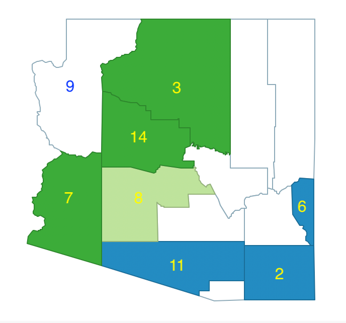
Figure 11.22: Arizona max-p growth phase - region 1, 2, 3
The next random seed yields county 9, with a population of 93,497. Its neighbors are already part of a previously assigned region (see Figure 11.22), and because it has insufficient population, county 9 cannot be turned into a region itself. Therefore it is relegated to the enclave.
The following random pick yields county 12, with a population of 116.379, and with as neighbors counties 4, 8, 11 and 5, as shown in Figure 11.23. Of the neighbors, counties 8 and 11 are already part of other regions, so they cannot be considered.
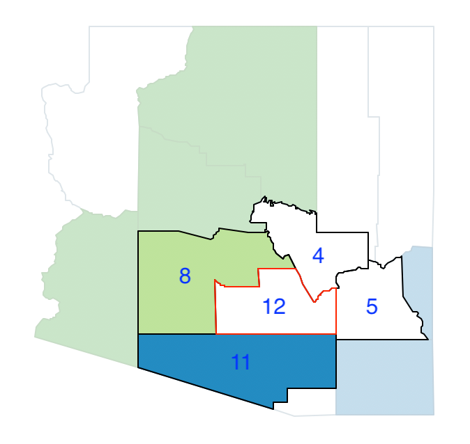
Figure 11.23: Arizona max-p growth phase - pick 12
Of the two neighbors of county 12, county 4 has the largest population, at 40,216, so it is joined with county 12. However, their total population of 156,595 does not meet the threshold, so additional neighbors need to be considered as. Of the six neighbors of county 4, that can be included in the neighbor list, only county 10 is an addition, shown in Figure 11.24.
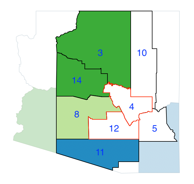
Figure 11.24: Arizona max-p growth phase - join 12 and 4
Between counties 5 and 10, the latter has the largest population (120,739), which brings the total for the region 12-4-10 to 277,334. The new configuration with four regions is shown in Figure 11.25, which now sets \(p=4\).
There are four remaining counties. County 9 is already in the enclave. Clearly, county 13 with a population of 29,676 is not large enough to form a region by itself, so it is added to the enclave as well.
Similarly, the combination of counties 5 and 1 only yields a total population of 88,145, which is insufficient to form a region, so they are both included in the enclave.
At this point, the growth phase has been completed and yielded \(p=4\), with four counties left in the enclave, as in Figure 11.25. In a typical application, this process would be repeated many times and only the solutions would be kept that achieve the largest \(p\). For those layouts, the best feasible initial solution must be obtained, in which all units are assigned to regions. Therefore, the counties that remain in the enclave must be assigned to one of the existing regions such as to minimize the total within sum of squares.
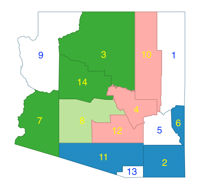
Figure 11.25: Arizona max-p enclaves and initial regions 1, 2, 3, 4
In the example, the solution is straightforward for counties 9 and 13: county 9 is merged with 3-14-7, and county 13 is merged with 11-2-6. For counties 5 and 1, the situation is a bit more complicated, since both could be assigned to either cluster 1 (2-6-11-13) or cluster 4 (4-10-12), or one to each, for a total of four combinations.
The calculations of the respective sum of squared deviations are listed in Figure 11.26. The starting point is a total SSD between cluster 1 and 4 of 1.7899, at the top of the Figure. Next, the new SSD is computed for the case where county 1 is added to the first cluster and county 5 to the fourth, and vice versa. This increases the total SSD between the two clusters to respectively 9.1762 and 6.5476. Finally, the scenarios where both county 1 and county 5 are added either to the first or to the fourth cluster are considered. The results for the new SSD are, respectively, 9.1840 and 6.2903.
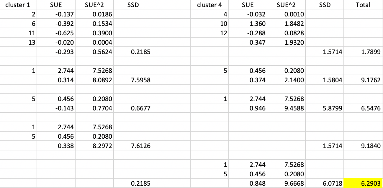
Figure 11.26: Arizona max-p assign enclaves
Consequently, the allocation that obtains the smallest within sum of squares is the regional configuration that assigns both counties 1 and 5 to region 4, shown in Figure 11.27. The constituting regions are 11-13-2-6, 8, 3-14-7-9, and 1-10-4-12-5.
At this point, there is a feasible initial solution that can form the starting point for one of the three search algorithms, in the same fashion as for AZP.
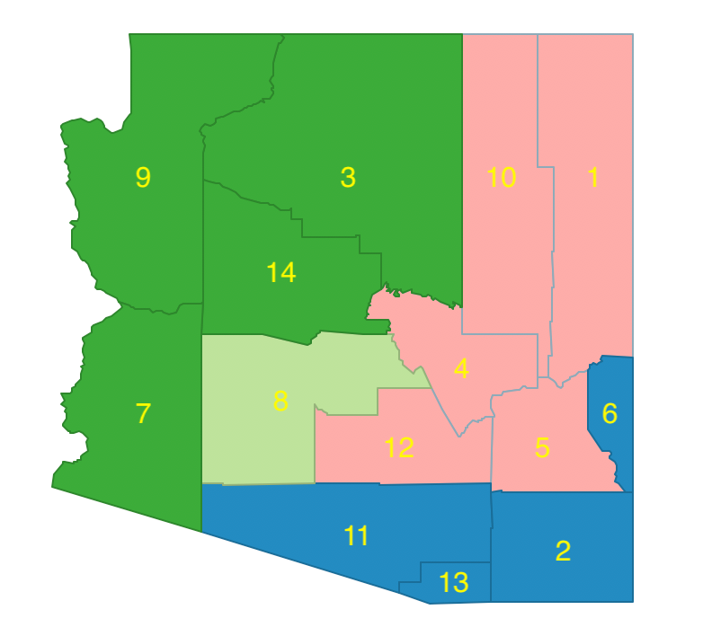
Figure 11.27: Arizona max-p - feasible initial regions
11.3.2 Implementation
The max-p option is available from the main menu as Clusters > max-p, or from the drop down list associated with the cluster toolbar icon, as the second item in the subset highlighted in Figure 11.1.
The variable settings dialog is again largely the same as for the other cluster algorithms, with the additional requirement to select a Mininum Bound variable and specify a threshold value. The same three Local Search options are available as for AZP. The default #iterations is set to 99.
From the drop down list, the variable for the Minimum Bound is selected as pop, the total population in each municipality. Its default setting is 10% of the total over all observations (i.e., the total population of the state of Ceará), which amounts to 845,238.
With all the default settings (and Greedy as the local search), the max-p solution only yields 6 regions, with a dismal BSS/TSS ratio of 0.2756. The main culprit is the highly skewed distribution for population size, with a median population of 19,970 for the municipalities. However, eight municipalities have a population greater than 100,000. The default setting is thus not a reasonable population threshold.
Some experimenting suggests a bound of 5% (422,619). With the number of iterations set to 9999 (higher values tend to yield better solutions), and using simulated annealing for the search, with a cooling rate of 0.9 and maxit=5 yields a max-p of 12. This turns out (purely by coincidence) to be the same number of regions as used in the previous examples, which makes the results comparable.
The overall fit is somewhat poorer, with a BSS/TSS ratio of 0.3846. In essence, this is the price to pay for imposing a minimum bound on the solution. The results are shown in Figure 11.28. In contrast to previous layouts, the cluster map is much more balanced, with only two smaller regions and no singletons.
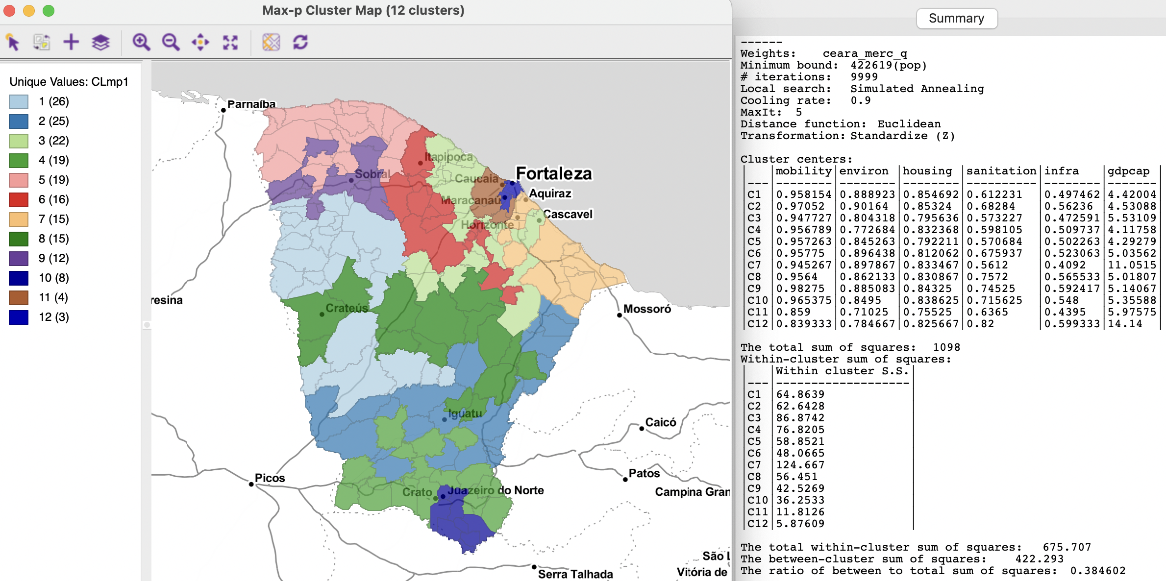
Figure 11.28: Ceará max-p regions with population bound 422,619
11.3.3 Sensitivity Analysis
The results of max-p are very sensitive to several parameters. Not only does the type of local search affect the results, but the number of iterations is very important, as is the minimum bound. When the latter is not based on a substantive concern (such as legal mandates), experimenting with different bounds will provide insight into the maximum \(p\) that can be obtained. For example, with the bound set at 3% of the total population, or 253,571, 19 clusters can be obtained (using simulated annealing with cooling rate 0.9, maxit=5 and 9999 iterations), shown in Figure 11.29. This yields a BSS/TSS ratio of 0.4389.
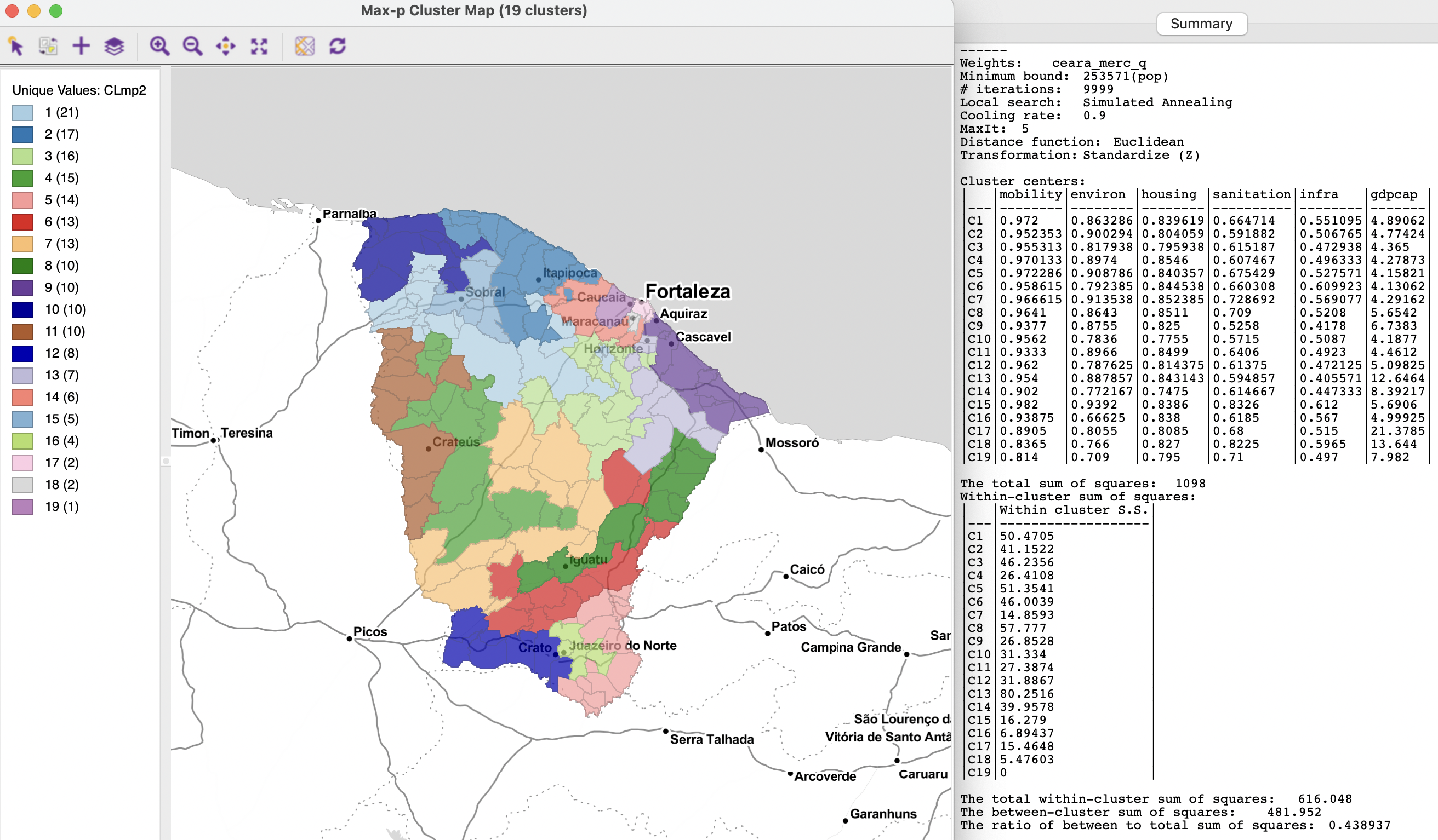
Figure 11.29: Ceará max-p regions with population bound 253,571
The solution of spatially constrained partitioning cluster methods is based on heuristics, which require substantial fine tuning. While this may seem disconcerting at first, it also provides the opportunity to gain closer insight into the various trade-offs involved. These include not only the tension between locational and attribute similarity, but also between the spatial characteristics of the resulting cluster map and the quantitative measures of fit. This is considered more closely in the final chapter.