9.4 Weighted Optimization of Geographical and Attribute Similarity

In the previous section, each variable was weighted equally when including geographic coordinates among the features in the clustering exercise. In contrast, in a weighted optimization, the coordinate variables are treated separately from the regular attributes, in the sense that the problem is now formulated as having two objective functions. One objective is focused on the similarity of the regular attributes (e.g., the six urban indicator variables), the other on the similarity of the geometric centroids. A weight changes the relative importance of each objective.

Early formulations of the idea behind a weighted optimization of geographical and attribute features can be found in Webster and Burrough (1972), Wise, Haining, and Ma (1997), and Haining, Wise, and Ma (2000). More recently, some other methods that have a soft enforcing of spatial constraints can be found in Yuan et al. (2015) and Cheruvelil et al. (2017), applied to spectral clustering, and in Chavent et al. (2018) for hierarchical clustering. In these approaches a relative weight is given to the dissimilarity that pertains to the regular attributes and one that pertains to the geographic coordinates. As the weight of the geographic part is increased, more spatial forcing occurs.

The approach outlined here is different, in that the weights are used to rescale the original variables in order to change the relative importance of attribute similarity versus locational similarity. This is a special case of weighted clustering, which is an option in several of the standard clustering implementations. The objective is to find a contiguous solution with the smallest weight given to the X-Y coordinates, thus sacrificing the least with respect to attribute similarity.

Consider there to be \(p\) regular attributes in addition to the X-Y coordinates. With a weight of \(w_1 \leq 1\) for the geographic coordinates, the weight for the regular attributes as a whole is \(w_2 = 1 - w_1\). These weights are distributed over the variables to achieve a rescaling that reflects the relative importance of space vs. attribute.

Specifically, the weight \(w_1\) is allocated to X and Y with each \(w_1/2\), whereas the weight \(w_2\) is allocated over the regular attributes as \(w_2/p\). For comparison, and using the same logic, in the method outlined in the previous section, each variable was given an equal weight of \(1/(p+2)\). In other words, all the variables, both attribute and locational were given the same weight.

The rescaled variables can be used in all of the standard clustering algorithms, without any further adjustments. One other important difference with the method in the previous section is that the X-Y coordinates are not taken into account to compute the cluster centers and assess performance measures. Those are based on the original unweighted attributes.

While the principle behind this approach is intuitive, it does not always work in practice, since the contiguity constraint is not actually part of the optimization process. Therefore, there are situations where simple re-weighting of the spatial and non-spatial attributes does not lead to a contiguous solution.

For all methods except spectral clustering, there is a direct relation between the relative weight given to the attributes and the measure of fit (e.g., the between to total sum of squares). As the weight for the X-Y coordinates increases, the fit on the attribute dimension will become poorer. However, for spectral clustering, this is not necessarily the case, since this method is not based on the original variables, but on a projection of these (the principal components).

In other words, the X-Y coordinates are used to pull the original unconstrained solution towards a point where all clusters consist of contiguous observations. Only when the weight given to the coordinates is small is such a solution still meaningful in terms of the original attributes. A large weight for the X-Y coordinates in essence forces a contiguous solution, similar to what would follow if only the coordinates were taken into account. While this obtains contiguity, it typically does not provide a meaningful result in terms of attribute similarity.

9.4.1 Optimization

The spatial constraint can be incorporated into an optimization process. In the heuristic outlined here, a bisection search is employed to find the cluster solution with the smallest weight for the X-Y coordinates that still satisfies a contiguity constraint. In most instances, this solution will also have the best fit of all the possible weights that satisfy the constraint. For spectral clustering, the solution only guarantees that it consists of contiguous clusters with the largest weight given to the original attributes.

The heuristic contains two important steps: changing the weight at each iteration in an efficient manner, and assessing whether the solution consists of contiguous clusters.

A limitation of this approach is that it does not deal well with isolates (islands), i.e., disconnected observations. Consequently, only results that designate the isolate(s) as separate clusters will meet the contiguity constraint. In such instances, it may be more practical to remove the isolate observations before carrying out the analysis.

The method outlined in the previous section implements soft spatial clustering, in the sense that not all clusters consist of spatially contiguous observations. In contrast, the approach outlined here enforces a hard spatial constraint, although possibly at the expense of a poor clustering performance for the attribute variables.

The point of departure is a purely spatial cluster that assigns a weight of \(w_1 = 1.0\) to the X-Y coordinates. This yields a set of spatially compact clusters for the given value of \(k\). Next, \(w_1\) is set to 0.5 and the contiguity constraint is checked. As is customary, contiguity is defined by a spatial weights specification. The spatial weights are represented internally as a graph. For each node in the graph, the algorithm keeps track of what cluster it belongs to.

If the contiguity constraint is satisfied for \(w_1 = 0.5\), that means that \(w_1\) can be further decreased, to get a better fit on the attribute clustering. Using a bisection logic, the weight is set to 0.25 and the contiguity constraint is checked again.

In contrast, if the contiguity constraint is not satisfied at \(w_1 = 0.5\), then the weight is increased to the mid-point between 0.5 and 1.0, i.e., 0.75, and the process is repeated. Each time, a failure to meet the contiguity constraint increases the weight, and the reverse results in a decrease of the weight. Following the bisection logic, the next point is always the midpoint between the current value and the closest previous value to the left or to the right. This process is continued until the change in the weight is less than a given tolerance.

In an ideal situation (highly unlikely in practice), \(w_1 = 0\) and the original cluster solution satisfies the spatial constraints. In the worst case, the search yields a weight \(w_1\) close to 1.0, which implies that the attributes are essentially ignored. More precisely, this means that the contiguity constraint cannot be met jointly with the other attributes. Only a solution that gives all or most of the weight to the X-Y coordinates meets the constraint.

In practice, any final solution with a weight larger than 0.5 should be viewed with skepticism, since it diminishes the importance of attribute similarity. Also, it is possible that the contiguity constraint cannot be satisfied unless (almost) all weight is given to the coordinates. This implies that a spatial contiguous solution is incompatible with the underlying attribute similarity for the given combination of variables and number of clusters (\(k\)). The spatially constrained clustering approaches covered in the next two chapters address this tension directly.

9.4.1.1 Connectivity check

In order to check whether the elements of a cluster are contiguous, an efficient search algorithm is implemented, essentially a breadth first search. The algorithm is of complexity O(n), which ensures that it scales well to large data sets.

The search starts at a random node and identifies all of the neighbors of that node that belong to the same cluster. Technically, the node IDs are pushed onto a stack. In this process, neighbors that are not part of the same cluster are ignored (i.e., they are not pushed onto the stack). Each element on the stack is examined in turn. If it has neighbors in the cluster that are not yet on the stack, they are added. Otherwise, nothing needs to be changed. After this evaluation, the node is popped from the stack. When the stack is empty, this means that all contiguous nodes have been examined.

At that point, if there are still unexamined observations in the cluster, i.e., if there are cluster members that are not in the current neighbor list, they must be unconnected. Therefore, the cluster is not contiguous and the process stops. In general, the examination of nodes is carried out until contiguity fails. If all nodes are examined without a failure, all clusters must consist of contiguous nodes (according to the definition used in the spatial weights specification). Since the algorithm is linear in the number of observations, it scales well.

To illustrate this process, consider the partial connectivity graph in Figure 9.6, based on the results for K-Means, shown in the left-hand panel of Figure 9.3. The neighbor structure is shown for the 17 members of C6, based on queen contiguity. This cluster consists of 12 unconnected subclusters, ranging in size from one to five elements.

If the random selection results in one of the singletons being picked, the check would be completed immediately, since those observations only have connections to locations outside the cluster. Since the remaining observations have not been visited, the cluster is clearly not contiguous.

The process is only slightly more complex if the random start is an observation from one of the other groups that consist of multiple elements. In each instance, once the connections to the within group members have been checked, it is clear that the set of 17 observations has not be exhausted, so that the contiguity constraint fails. Once the contiguity constraint is not met for one of the clusters, there is no use in examining other clusters and the search stops.

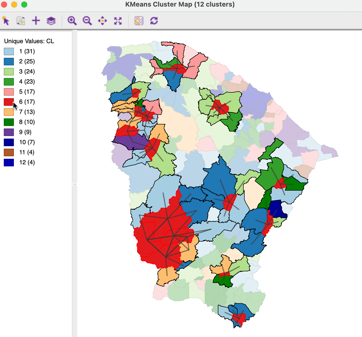
Figure 9.6: Connectivity Check for Cluster Members

9.4.2 Implementation

The weighted clustering is invoked in the same manner for each of the five standard clustering techniques. Just below the list of variables in the Clustering Settings interface, there is a check box next to Use geometric centroids. The default setting is Auto Weighting, which will run the bisection search. Alternatively, a Weighting can be specified using a slider bar or by entering a numerical value (the default is 1.00). The coordinates of the spatial units do not need to be specified in the variable list. They are calculated under the hood. As before, a warning is generated when the projection information is invalid.

In addition, a spatial weights file needs to be specified. This is used to assess the spatial constraint. In the absence of a weights file, a warning is generated. In the illustration, the weights file is for queen contiguity. The other six variables are the same as in the previous examples.

To illustrate the process, consider a K-Means clustering application. Before computing the clusters, the Auto Weighting button must be clicked to find the solution of the bisection search. In this application, the resulting weight is 0.890015, clearly much larger than 0.5. As a consequence, the clusters may be spatially contiguous, but they will largely ignore the attribute similarity.

The resulting cluster map is shown in Figure 9.7. The clusters are clearly contiguous and their spatial layout shows a strong resemblance to the coordinate-based clusters in the left-hand panel of Figure 9.1. On the other hand, they do not match the spatial pattern of the pure K-Means result in the left-hand panel of Figure 9.3, except to some extent for the central region and the region around the city of Fortaleza.

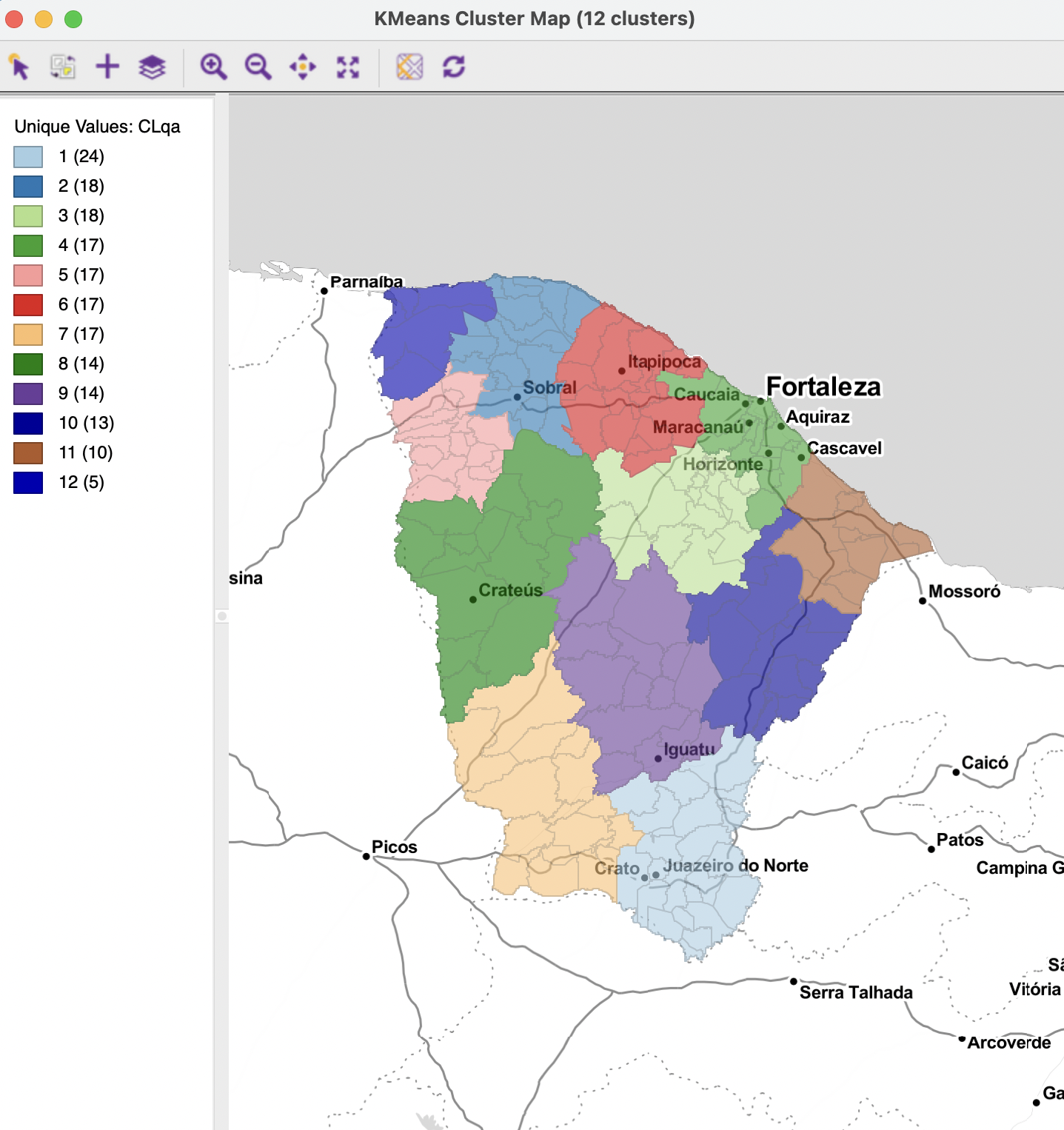
Figure 9.7: Cluster Map, K-Means with Weighted Optimization

The cluster characteristics are given in Figure 9.8. They include the weights for the variables, i.e., 0.445 for each of the coordinates and 0.01833 for each of the six socio-economic attributes. The overall fit of the cluster on the attributes (the coordinates are not included in this calculation) is a pretty dismal BSS/TSS ratio of 0.247, compared to the unrestricted K-Means result of 0.682. This highlights the difficulty in fusing the objectives of attribute similarity and locational similarity.

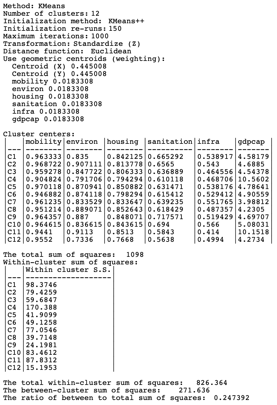
Figure 9.8: Cluster Characteristics, K-Means with Weighted Optimization

As mentioned in the discussion of the cluster characteristics with an augmented feature set, the X and Y coordinates are included in the computation of the cluster centers and the various measures of fit. The resulting BSS/TSS ratio is therefore not directly comparable with the results from the original K-Means. Since the augmented approach boils down to using equal weights for all variables, the corresponding weights for the coordinates together are 1/8 + 1/8 = 0.250.

The results of the cluster map in the right-hand panel in Figure 9.3 can be replicated by setting the Weighting to 0.25. The cluster map is identical to the one in Figure 9.3, but the cluster characteristics are not. They are listed in Figure 9.9. The variable weights are 0.125 (1/8) each, and the resulting cluster centers no longer include the information on the X-Y coordinates. The BSS/TSS ratio is now directly comparable to the standard K-Means results. At 0.585, a decrease from 0.682, it shows the price to pay for the spatial nudging, even though the end result is not contiguous.

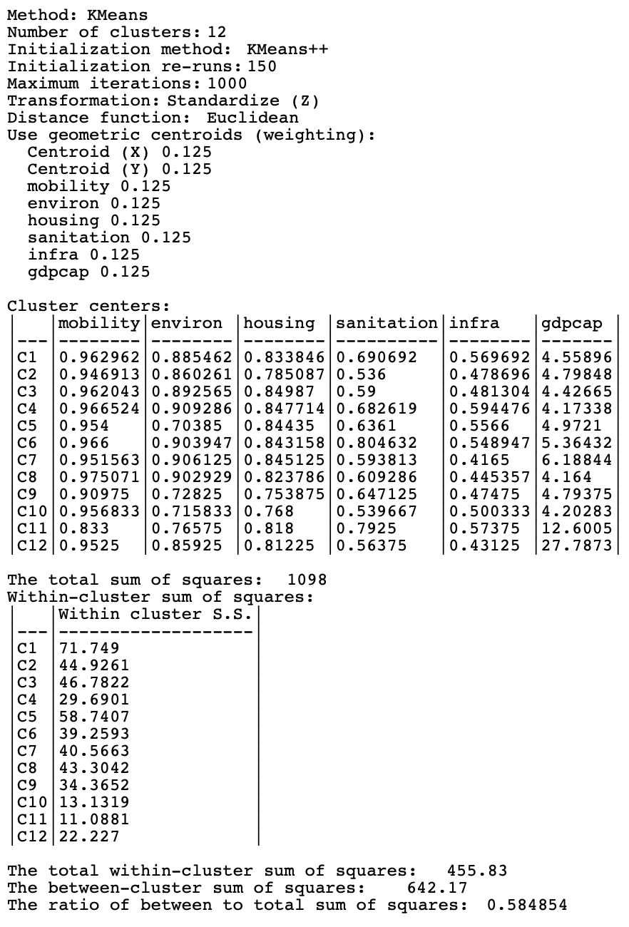
Figure 9.9: Cluster Characteristics, K-Means with Weights at 0.25