12.2 Internal Validity
Indices pertaining to the internal validity of a cluster focus on the composition of the clusters in terms of how homogeneous the observations are, how well clusters find the right separation between groups, as well as the balance among individual cluster sizes.
Five types of measures are considered here. First are traditional measures of fit that were included among the Summary of cluster characteristics in the preceding chapters. Next follow indicators of the balance of cluster sizes, i.e., the evenness of the number of observations in each cluster.
The final three types of measures are less common. The join count ratio is an indicator of the compactness and separation between clusters in terms of the number of connections with observations outside the cluster. Compactness is a characteristic of the shape of a spatially constrained cluster and can be assessed by many different indicators. Finally, connectedness is an alternative measure of compactness that is derived from the graph structure of the spatial weights.
12.2.1 Traditional Measures of Fit
As covered in previous chapters, the total sum of squared deviations from the mean (TSS) is decomposed into one part attributed to the within sum of squares (WSS) and a complementary part due to the between sum of squares (BSS). These are the most commonly used indicators of the fit of a clustering to the data. A better cluster is considered to be one with a smaller WSS, or, equivalently, a larger BSS to TSS ratio. As noted earlier, this is only an appropriate metric when the dissimilarity matrix is based on an Euclidean distance. When this is not the case, e.g., for K-Medoids, a different metric should be used.
While useful, these indicators of fit miss other important characteristic of a cluster. For example, in order to better identify critical assignments within a given cluster alignment, Kaufman and Rousseeuw (2005) introduced the notion of average silhouette width. This is the average dissimilarity of an observation to members of its own cluster compared to the average dissimilarity to observations in the closest cluster to which it was not classified. An extension that takes the spatial configuration into account in the form of so-called geo-silhouettes is presented in Wolf, Knaap, and Rey (2021).
12.2.2 Balance
In many applications, it is important that the clusters are of roughly equal size. Two common indicators are the entropy and Simpson’s index. Both compare the distribution of the number of observations among clusters to an even distribution. Whereas entropy is maximized for such a distribution, Simpson’s index is minimized.
The entropy for a given clustering \(P\) consisting of \(k\) clusters with observations \(n_i\) in cluster \(i\), for a total of \(n\) observations, is (see, e.g., Vinh, Epps, and Bailey 2010): \[H(P) = - \sum_{i=1}^k \frac{n_i}{n} \log \frac{n_i}{n}.\] For equally balanced clusters, \(n_i/n = 1/k\), so that entropy is \(- k .(1/k) \ln(1/k) = ln(k)\), which is the maximum that can be obtained for a given \(k\). To facilitate comparison among clusters of different sizes, a standardized measure can be computed as entropy/max entropy. The closer this ratio is to 1, the better the cluster balance (by construction, the ratio is always smaller than 1).
The entropy fragmentation index can be computed for the overall cluster result, but also for each cluster separately. This is especially relevant when a cluster consists of subclusters, i.e., subsets of contiguous observations. A cluster that consists of subclusters of equal size would have a relative entropy of 1. The sub-cluster entropy is only a valid measure for non-contiguous or non-compact clusters, so it is not appropriate for the results of spatially constrained clustering methods.
Another indicator of cluster balance is Simpson’s index of diversity (Simpson 1949), also known in economics as the Herfindahl-Hirschman index: \[S = \sum_{i=1}^k (\frac{n_i}{n})^2.\] With equal representation in clusters, Simpson’s index equals \(1/k\), the lowest possible value. It ranges from \(1/k\) to \(1\) (all observations in a single cluster). A standardized index yields a value of 1 for the equal representation case, and values larger than 1 for others, with smaller values indicating a more balanced distribution.55
Same as for the entropy measure, Simpson’s index is only applied to subclusters in cases where the solution is not spatially constrained.
12.2.3 Join Count Ratio
An index that addresses both compactness and separation is the join count ratio. It is derived from the contiguity structure among observations that is reflected in a spatial weights matrix. For a given such structure, a relative measure of compactness of a cluster is indicated by how many neighbors of each observation in the cluster are also members of the cluster. For a spatially compact cluster, ignoring border effects, this ratio should be 1. The higher the ratio, the more compact and self-contained is the cluster, with the least connectivity to other clusters.
The join count ratio can be computed for each cluster separately, as well as for the clustering as a whole. A value of zero (the minimum) indicates that all neighbors of the cluster members are outside the cluster. This is only possible when the cluster is not spatially constrained and when all cluster elements are singletons in a spatial sense.
12.2.4 Compactness
For spatially constrained clusters, compactness is a key characteristic. For example, this is a legal criterion in the context of electoral redistricting, which is a form of spatially constrained clustering (Saxon 2020). However, there is no single measure to characterize compactness, and many different aspects of the shape of clusters can be taken into account (e.g., the review in Niemi et al. 1990). For example, Saxon (2020) reviews no less than 18 indicators of compactness and compares their properties in the context of gerrymandering..
Perhaps the most famous measure of compactness is the isoperimeter quotient (IPQ), i.e., the ratio of the area of a cluster shape to that of a circle of equal perimeter (Polsby and Popper 1990).
The point of departure is the view that a circle is the most compact shape. It is compared to an irregular polygon with the same perimeter.56 The area of a circle, expressed in function of its perimeter \(p\) is \(C = p^2 / 4\pi\).57 Consequently, the isoperimeter quotient as the ratio of the area of the polygon \(A\) over the area of the circle is: \[IPQ = 4 \pi A / p^2,\] with \(A\) as the area of the polygon.
The IPQ is only suitable for spatially constrained cluster results.
12.2.5 Connectedness
With the spatial weights viewed as a network or graph, a spatially constrained cluster must constitute a so-called connected component. The diameter of the network structure that corresponds with the cluster is the length of the longest shortest path between any pair of observations (Newman 2018, 133). Starting from an unweighted graph representation of the spatial weights matrix, each connection between two neighbors corresponds with one step in the graph.
For a given number of observations in a cluster, the diameter computed from the spatial weights connectivity graph gives a measure of compactness (smaller is more compact). For example, for a star-shaped layout of observations, the diameter would equal two (the longest shortest path between any pair of observations goes through the center of the star in two steps). On the other end of the spectrum, for a long string of \(m\) observations, the diameter would be \(m-1\).
Everything else being the same, the diameter of a network increases with its size. Dividing the diameter by the number of observations in the cluster gives a relative measure, which corrects for the size of the cluster.
As for the IPQ, the diameter of a cluster is only applicable to spatially constrained clusters.
12.2.6 Implementation
To compare the different cluster validation measures, eight different outcomes are considered, all obtained with \(k=12\) for the Ceará economic indicators (\(n = 184\)). Two clusterings are non-spatial, i.e., Hierarchical clustering with Ward’s linkage (not used earlier, but shown in Figure 12.2 below), and K-Means (cluster map in the left-hand panel of Figure 9.3, characteristics in Figure 9.4). The remaining six patterns represent different methods to obtain spatially constrained results: SCHC with Ward’s linkage (Figure 10.10 and Figure 10.11); SKATER (Figure 10.18 and Figure 10.19); REDCAP (Figure 10.24 and Figure 10.25); AZP with simulated annealing (Figure 11.12); AZP with SCHC as initial solution (Figure 11.14); and the max-p outcome that yielded \(p=12\) (Figure 11.28).
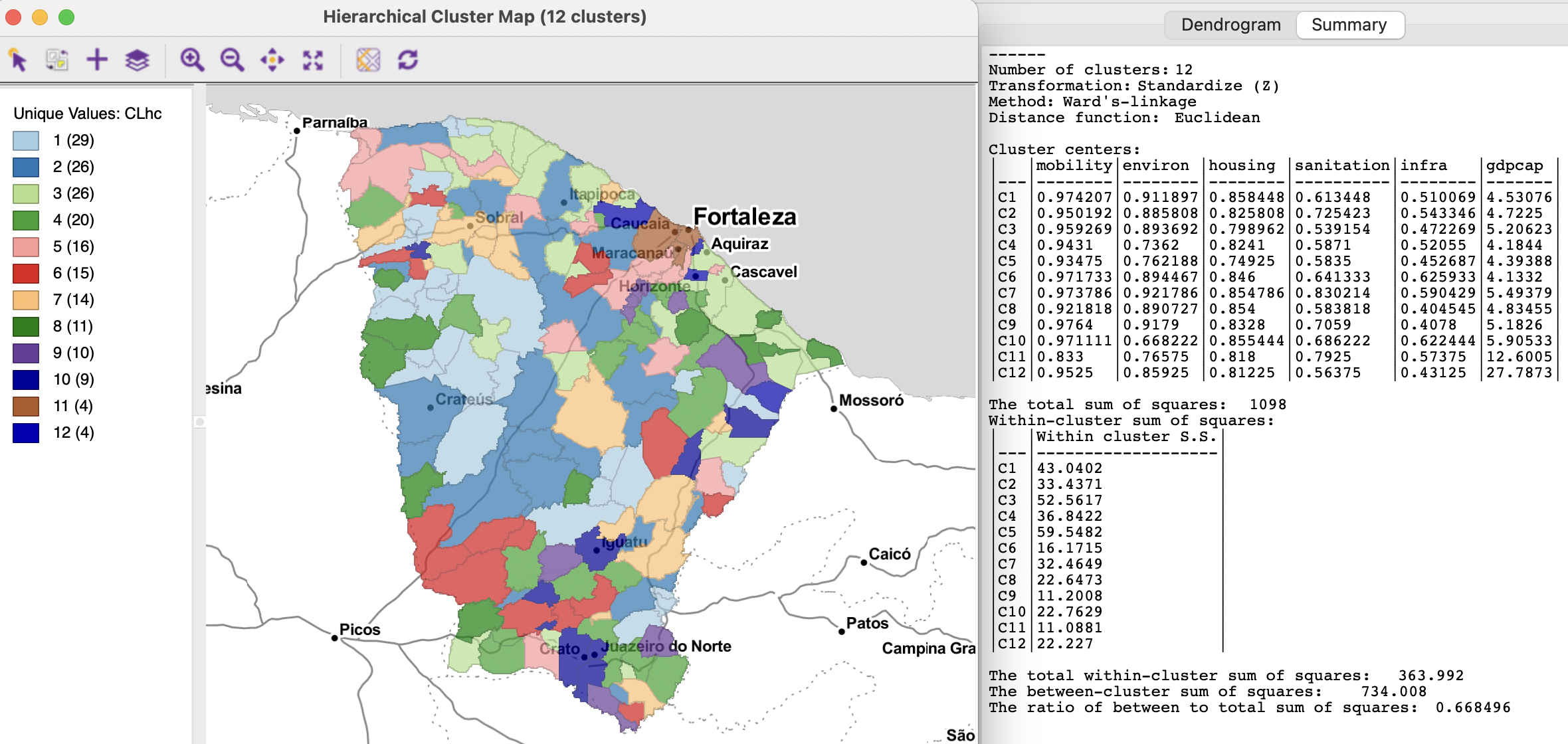
Figure 12.2: Hierarchical Clustering - Ward’s method, Ceará
The WSS, BSS/TSS ratio, overall Entropy, Simpson’s index and the join count ratio for each clustering are listed in Figure 12.3. The first two measures are included as part of the Summary for each cluster result. The others are invoked by selecting Clusters > Validation from the menu, or as the last item in the cluster drop-down list from the toolbar (see Figure 12.1). The required input is a Cluster Indicator (i.e., the categorical variable saved when carrying out a clustering exercise) and a spatial weights file. The latter is required for the join count ratio, even for traditional (non-spatial) clustering methods.

Figure 12.3: Internal Validation Measures
The Validation option brings up a results window, shown in Figure 12.4 for the hierarchical clustering outcome. At the top, this gives the number of clusters (12), the raw and standardized entropy measures as well as the raw and standardized Simpson’s index.
Since the hierarchical cluster outcome is not spatially constrained, the fragmentation characteristics are also listed for each of the twelve clusters individually. The size is given (N), its share in the total number of observations (Fraction), the number of sub-clusters (#Sub), raw and standardized Entropy and Simpson index, as well as the minimum, maximum and mean size of the subclusters. This provides a detailed picture of the degree of fragmentation by cluster. For example, the table shows that cluster 11 consists of 4 compact observations (fragmentation results given as 0), whereas cluster 12 is made up of 4 singletons, the most fragmented result (yielding a standardized value of 1 for both entropy and Simpson’s index). The best result, in the sense of the least fragmentation or least diverse is obtained for cluster 1. Its 29 observations are divided among 9 subclusters (smallest standardized entropy, i.e., worst diversity, of 0.797 and largest standardized Simpson of 2.258).
In addition to the fragmentation measures, the join count ratio is computed for each individual cluster as well. This provides the number of neighbors and the count of joins that belong to the same cluster, yielding the join count ratio. At the bottom, the overall join count ratio is listed. Taking into account the neighbor structure yields cluster 11 (which has no subclusters, hence is compact) with the highest score of 0.476, closely followed by cluster 1 with 0.405.
Since the result pertains to a method that is not spatially constrained, there are no measures for compactness and diameter.
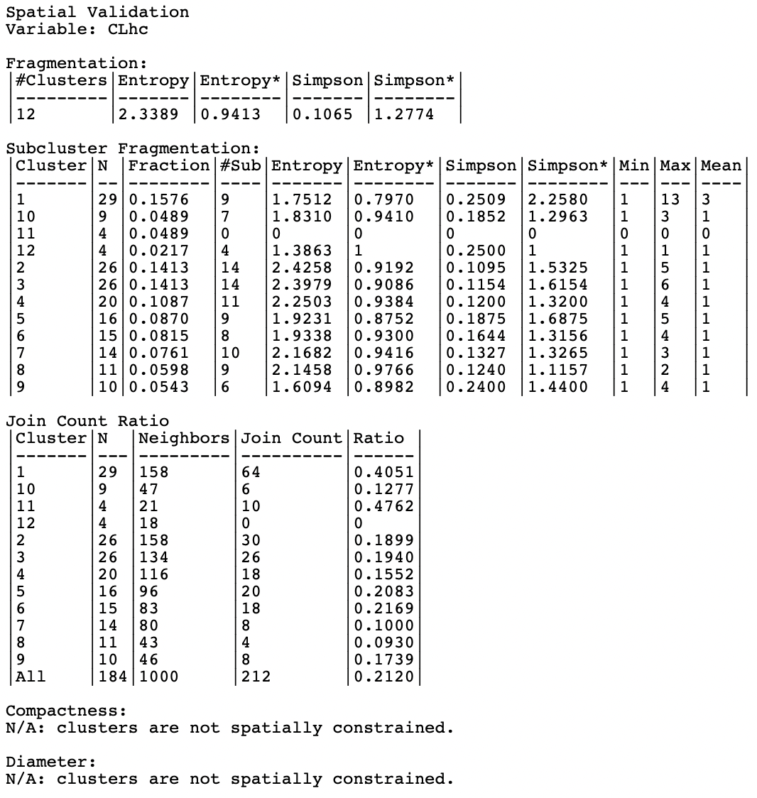
Figure 12.4: Internal Validation Result - Hierarchical Clustering
Comparing the overall results in Figure 12.3 confirms the superiority of the K-Means outcome in terms of fit, with the best WSS and BSS/TSS. In general, the unconstrained clustering methods do (much) better on these criteria than the spatially constrained results, with only AZP-initial coming somewhat close. This matches a similar dichotomy for the fragmentation indicators, with the spatially constrained outcomes much less equally balanced (smaller entropy, larger Simpson) than the classical results. Interestingly, the minimum population size imposed in max-p yields a more balanced outcome, with entropy and Simpson on a par with the classical results (but much worse overall fit). Finally, the overall join count ratio confirms the superiority of the spatially constrained results in this respect, with SKATER yielding the highest ratio.
For a spatially constrained clustering method, the results window for Validation is slightly different, as illustrated in Figure 12.5 for AZP with a SCHC initial region.
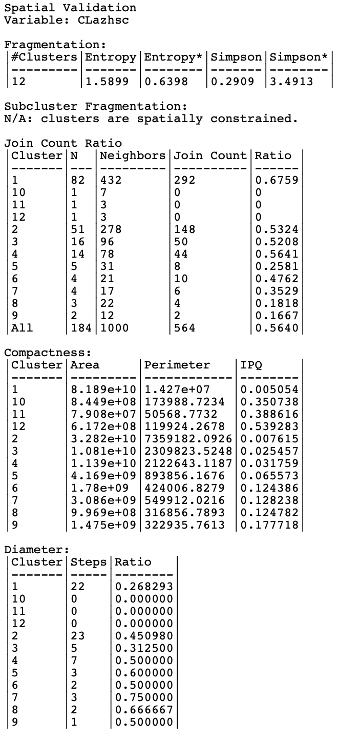
Figure 12.5: Internal Validation Result - AZP with Initial Region
The fragmentation summary takes the same form as before, but there is no report on subcluster fragmentation. The join count ratio is again included, with the outcome for all individual clusters as well as the overall ratio. In the example, the highest ratio is obtained in cluster 1, with a value of 0.6759, compared to the overall ratio of 0.564.
Two additional summary tables include the computation of the IPQ as a compactness index, as well as the diameter based on the spatial weights in each cluster.
The highest values for IPQ are obtained for the singletons, which is not very informative. Of the four largest clusters, cluster 4 (with 14 observations) seems the most compact, with a ratio of 0.032. Overall, the smaller clusters clearly do better on this criterion. For example, cluster 5 (with 5 observations) achieves a ratio of 0.066, and cluster 7 (with 4 observations) obtains a ratio of 0.128. For comparison, the largest ratio obtained for a singleton is for cluster 12, with a ratio of 0.539.
Finally, the diameter ranges from 0 (for singletons) to 23 for cluster 2 (with 51 observations). Standardized for the number of observations in each cluster, cluster 1 is most connected (22 steps with 82 observations, for a ratio of 0.286), closely followed by cluster 3, which is much smaller (16 observations with 5 steps, for a ratio of 0.3125).
Clearly, the different dimensions of performance highlight distinct characteristics of each cluster. In each particular application, some dimensions may be more relevant than others, requiring a careful assessment.
In the literature, a normalized Herfindahl-Hirschman index is sometimes used as (HHI - 1/n) / (1 - 1/n), which runs from 0 to 1, with 0 as best.↩︎
Technically speaking, determining the perimeter of an irregular polygon is not without problems, and depends on the precision of the digital representation of the boundary.↩︎
The perimeter of a circle is \(p = 2 \pi r\), with \(r\) as the radius, so \(r = p / 2\pi\). The area of a circle is \(C = \pi r^2\), so expressed as a function of the perimeter, it is \(C = \pi (p / 2\pi)^2 = p^2 / 4\pi\).↩︎