10.2 Spatially Constrained Hierarchical Clustering (SCHC)

Spatially constrained hierarchical clustering is a special form of constrained clustering, where the constraint is based on contiguity (common borders). In the discussion of classic clustering algorithms, a constrained approach was already considered when a minimum size was imposed. The spatial constraint is more complex in that it directly affects the way in which elemental units can be merged into larger entities.

The idea of including contiguity constraints into agglomerative hierarchical clustering goes back a long way, with early overviews of the principles involved in Lankford (1969), Murtagh (1985) and Gordon (1996). Recent software implementations can be found in Guo (2009) and Recchia (2010), among others.

The clustering logic is identical to that followed for unconstrained hierarchical clustering, and the same expressions are used for linkage and updating formulas, i.e., single linkage, complete linkage, average linkage, and Ward’s method (see Chapter 5 for details). The only difference is that a contiguity constraint is imposed, based on the non-zero elements of a spatial weights matrix (\(w_{ij} \neq 0\)).

More specifically, two entities \(i\) and \(j\) are merged when the dissimilarity measure \(d_{ij}\) is the smallest among all pairs of entities, subject to \(w_{ij} = 1\). In other words, merger is only carried out when the corresponding entry in the spatial weights (contiguity) matrix is non-zero. Another way to phrase this is that the minimum of the dissimilarity measure is only searched for those pairs of observations that are contiguous.

As before, the dissimilarity measure is recomputed for the newly merged unit using the appropriate formula. In addition, the weights matrix needs to be updated to reflect the contiguity structure of the newly merged units.

In the first step, the weights matrix is of dimension \(n \times n\). If observations \(i\) and \(j\) are merged into a new entity, say \(A\), then the resulting matrix will be of dimension \((n - 1) \times (n-1)\) and the two original rows/columns for \(i\) and \(j\) will be replaced by a new row/column for \(A\). For the new matrix, the row elements \(w_{Ah} = 1\) if either \(w_{ih} = 1\) or \(w_{jh} = 1\) (or both are non-zero), and similarly for the column elements.

The next step thus consists of a new dissimilarity matrix and new contiguity matrix, both of dimension \((n - 1) \times (n-1)\). At this point the process repeats itself. As for other hierarchical clustering methods, the end result is a single cluster that contains all the observations. The process of merging consecutive entities is graphically represented in an dendrogram, as before.

One potential complication is so-called inversion, when the dissimilarity criterion for the newly merged unit with respect to remaining observations is better than for the merged units themselves. This link reversal occurs when \(d_{i \cup j, k} < d_{ij}\). It is only avoided in the complete linkage case (for details, see Murtagh 1985; Gordon 1996). This problem is primarily one of interpretation and does not preclude the clustering methods from being applied.

10.2.1 The Algorithm

To illustrate the mechanics of the algorithm, a small worked example is provided, using the layout of the 14 counties in the U.S. state of Arizona, shown in Figure 10.2.

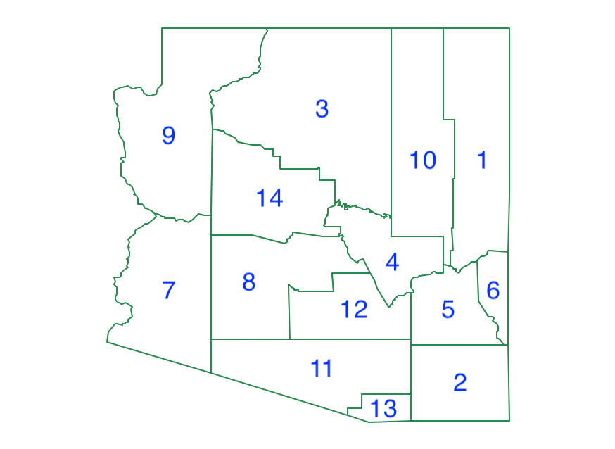
Figure 10.2: Arizona counties

To keep matters simple, only a single variable is used, listed in standardized form in Figure 10.3.⁴⁶

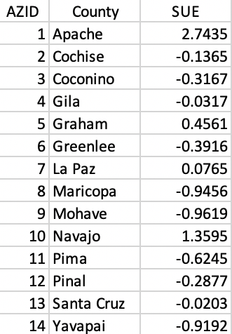
Figure 10.3: County identifiers and standardized variable

A final element is the spatial weights matrix, here implemented as first order queen contiguity, contained in Figure 10.4.

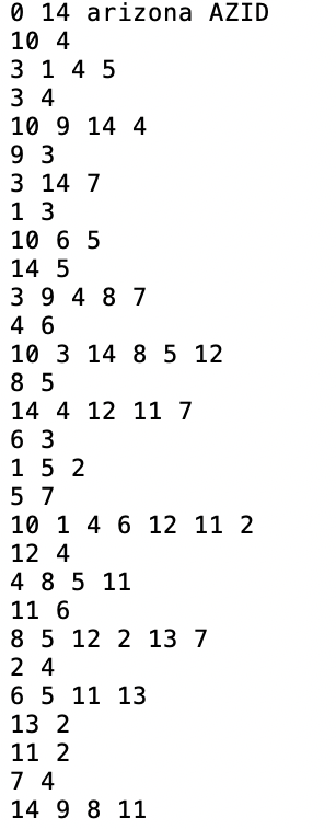
Figure 10.4: AZ county queen contiguity information in GAL file format

10.2.1.1 SCHC Complete Linkage

SCHC is implemented for four classic linkage functions. To keep the illustration simple, complete linkage is used, which tends to yield compact clusters with an easy updating formula (max distance). Even though this is not an ideal linkage selection, it is easy to implement and helps to illustrate the logic of the SCHC.

The point of departure is the matrix of Euclidean distance in attribute space. In the example, there is only one variable, so the distance is equivalent to the absolute difference between the values at two locations (the square root of the squared difference). In Figure 10.5, the full distance matrix is shown. Distinct from the example in the unconstrained case, attention is limited to those pairs of observations that are spatially contiguous, shown highlighted in red in the matrix.

The first step is to identify the pair of observations that are closest in attribute space and contiguous. Inspection of the distance matrix in Figure 10.5 finds the pair 8-14 as the least different, with a distance value of 0.03.

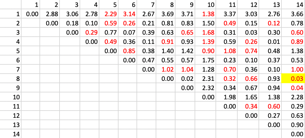
Figure 10.5: SCHC complete linkage step 1

The next step is to combine observations 8 and 14 and recompute the distance from other observations as the largest from either 8 or 14. The updated matrix is shown in Figure 10.6. In addition, the contiguity matrix must be updated with neighbors to the cluster 8-14 as those who were either neighbors to 8 or 14, or to both. The updated neighbor relation is shown as the red values in the matrix. The smallest distance value is between 9 and 8-14, which yields a new cluster of 8-9-14.

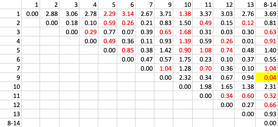
Figure 10.6: SCHC complete linkage step 2

The remaining steps proceed in the same manner. The contiguity relations are updated and the largest distance between the two elements of the cluster is entered as the new distance in the matrix.

The next step combines 2 and 13, followed by 4 and 12, etc.

The complete set of steps can be visualized in a dendrogram, shown in Figure 10.7. As before, the horizontal axis illustrates the change in objective function at each step, starting with the combination of 8 and 14, followed by adding 9, etc.

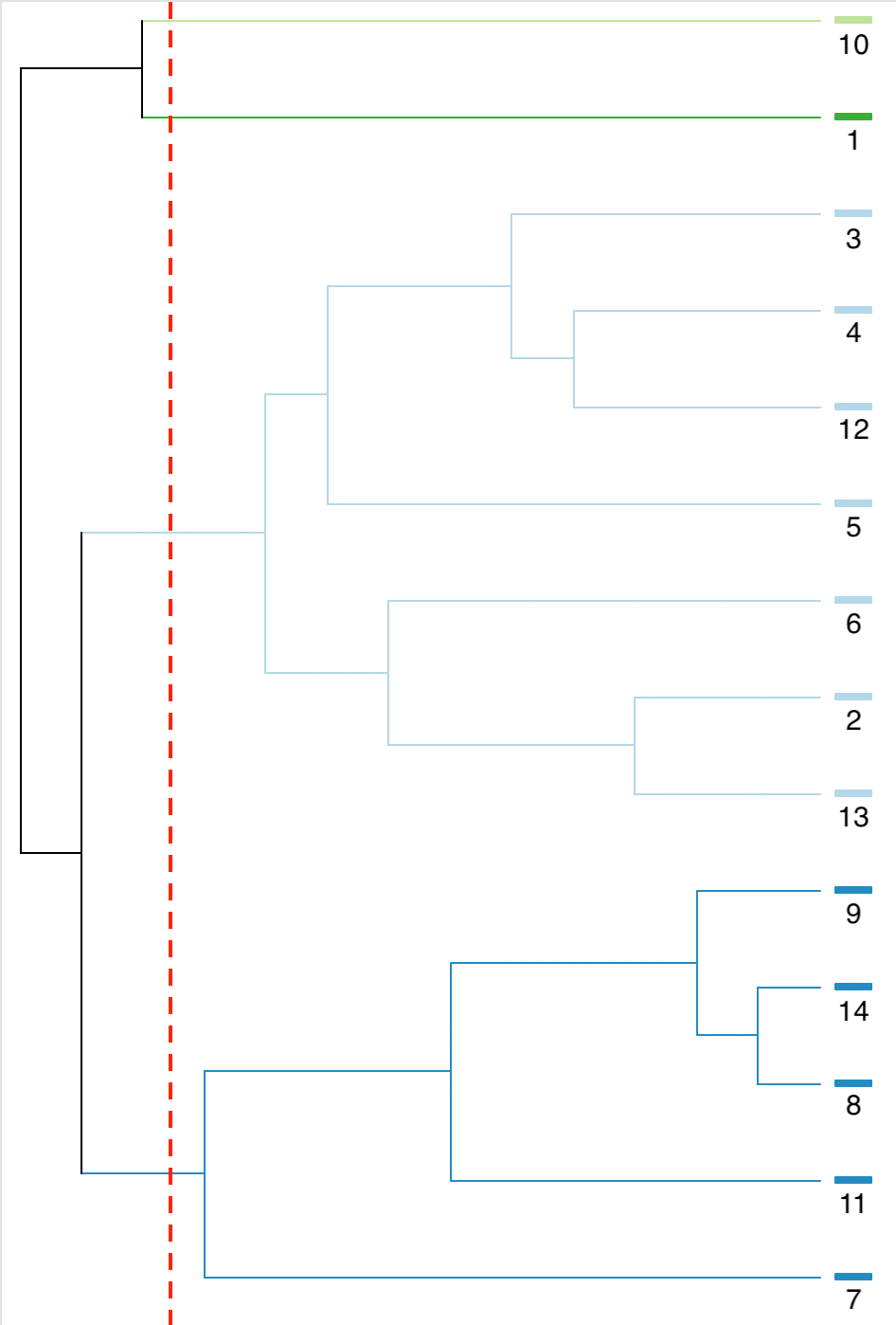
Figure 10.7: SCHC complete linkage dendrogram, k=4

The spatial layout of the clusters that results for a cut at k=4 is shown in Figure 10.8. Clearly, the contiguity constraint has been satisfied.

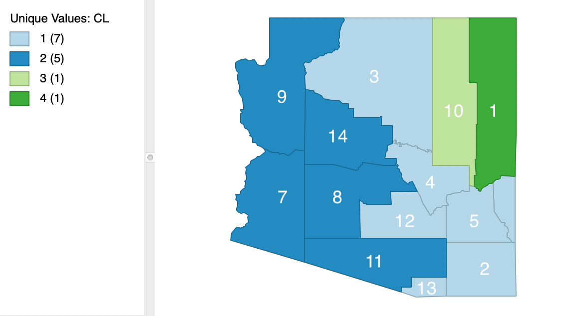
Figure 10.8: SCHC complete linkage cluster map, k=4

10.2.2 Implementation

The example is the same as in the previous chapter, using the 184 municipalities in the Brazilian state of Ceará and six socio-economic indicators: mobility, environ, housing, sanitation, infra and gdpcap. The spatial weights are based on first order queen contiguity.

Only Ward’s approach is illustrated, being the preferred linkage method (and the default). The other linkage methods are implemented in the same way, but typically result in worse cluster layouts, similar to what held for their unconstrained counterparts.

Spatially constrained hierarchical clustering is invoked from the drop down list associated with the cluster toolbar icon, as the first item in the subset highlighted in Figure 10.1. It can also be selected from the menu as Clusters > SCHC.

This brings up the Spatial Constrained Hierarchical Clustering Settings dialog, which consists of the two customary main panels, as was the case for classic hierarchical clustering.

The settings are shown in 10.9, with the left panel as the interface to specify the variables and a range of parameters, The right panel provides the results, either as a Dendrogram or as a tabular Summary, each invoked by a button at the top.

In the example, the six variables are selected, with all other items left to their default settings (see Section 5.4.1 for details), except for the location of the cut line, which is set to 12, consistent with the examples in the previous chapter. Also, the Method is kept to Ward’s-linkage, with the three other linkage methods available from the drop down list.

The resulting dendrogram is included on the right.

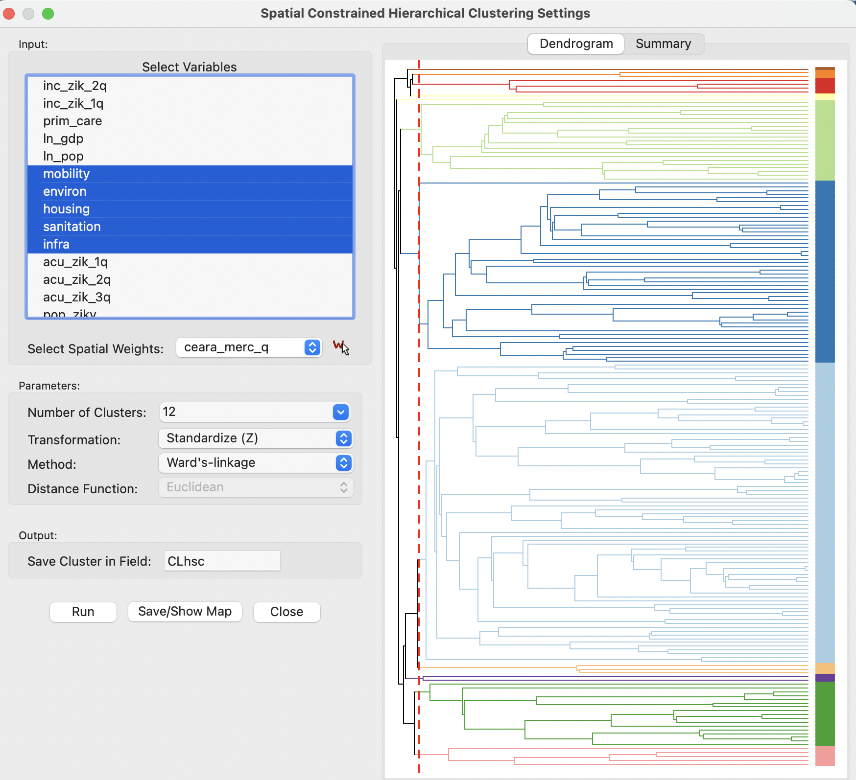
Figure 10.9: SCHC variable selection dialog

The corresponding cluster map is shown in Figure 10.10. It can be compared to the various cluster maps obtained in the previous chapter. In contrast to those cases, now the clusters all consist of contiguous units. However, the contiguity constraint has resulted in eight clusters out of the twelve to contain five or fewer observations, including three singletons. The largest cluster contains almost half the observations (79), the next one is half its size (48), and then again half the size (21). There are also some peculiar configurations that follow from the queen contiguity definition (common vertices). At first sight, the single municipality that belongs to cluster 2 (highlighted in the red square) seems like it should be part of cluster 3. However, it turns out to be connected to two municipalities in cluster 2 with a common vertex.

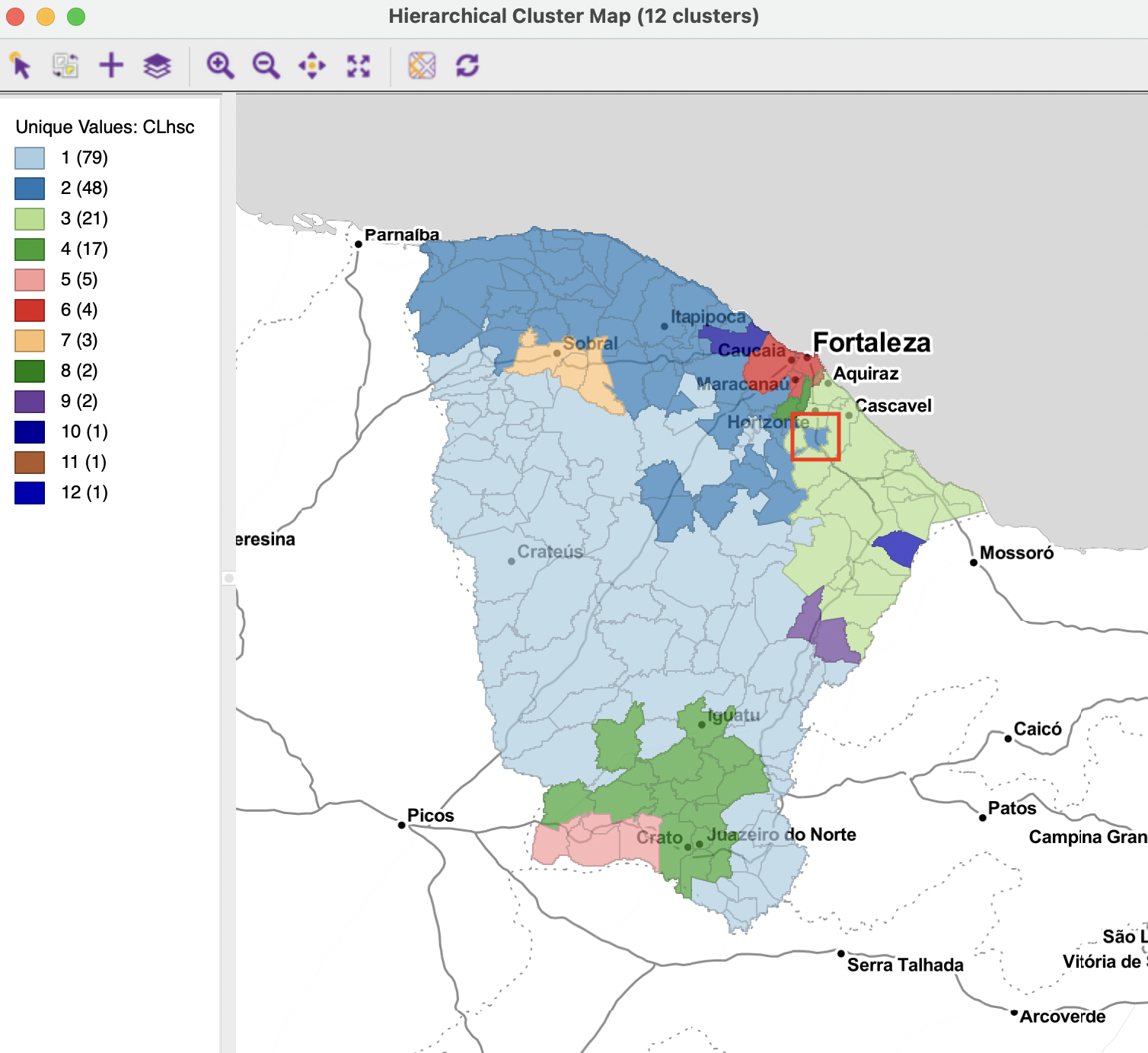
Figure 10.10: SCHC cluster map

The loss in cluster performance relative to K-means (see Figure 9.4) is again severe, though not quite as bad as in the examples of the previous chapter. The BSS/TSS ratio is 0.464, relative to 0.682 for K-means (see Figure 10.11).

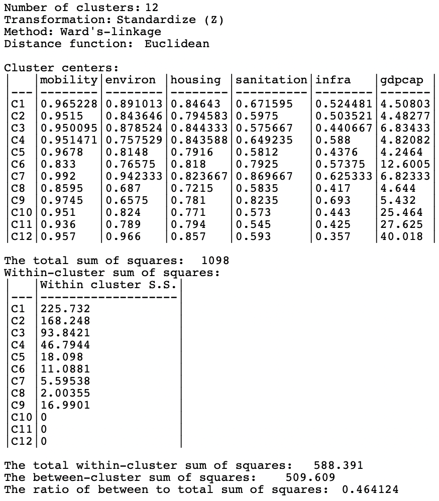
Figure 10.11: SCHC cluster characteristics

---

46. The variable is the standardized unemployment rate for 1990, from the natregimes GeoDa sample data set.↩︎