9.5 Constructing a Spatially Contiguous Solution

A final heuristic to illustrate the tension between attribute similarity and locational similarity constructs a contiguous spatial layout from an initial non-contiguous cluster solution. The heuristic only considers spatial aspects of the data, i.e., contiguity, and ignores the attribute values. Therefore, it will seldom yield an optimal solution. Nevertheless, it serves to illustrate the trade offs between the two objectives and provides a benchmark to compare to the spatially constrained solutions.

The principle behind the heuristic is to combine unconnected cluster subsets with the largest adjoining subcluster, until all clusters either are contiguous or consist of a singleton, respecting the original number of clusters, \(k\). As usual, the contiguity structure is defined by a spatial weights matrix.

The process starts with the smallest non-singleton cluster - singletons are left alone. If it consists entirely of contiguous elements, then it is left as is, and the next smallest cluster is considered. A non-contiguous cluster is a cluster that consists of two or more subcomponents. It is evaluated from small to large. Any singleton sub-clusters are assigned to the largest adjoining cluster. The same is done with any larger subcluster, moving from small to large until there is only one entity for that cluster class. When determining which is the largest adjoining cluster, the cluster elements are updated at each step.

The result for each unconnected cluster is that all its smallest elements are absorbed by other subclusters, until only a single entity remains.

To illustrate this process, consider the cluster map for the K-Means solution depicted in the left-hand panel of Figure 9.10. The smallest cluster, C12, consists of a set of four contiguous municipalities, so it does not need to be considered. The next smallest cluster, C11, consists of four singletons, shown as brown cells in the selection in the figure, highlighted within a red rectangle. Each singleton is considered in turn (in random order) and assigned to its largest adjoining cluster, until there is only one left (using queen contiguity to define adjoining cells). In the right-hand panel of the figure, the top-most singleton is assigned to cluster C3 (light green), the middle one to C5 (light rose), and the right-most one to C1 (light blue). The one by the coast is left as is. In this unique values map, the cluster category counts are adjusted accordingly. C11 now has only 1 member, C1 has 32, C3 25, and C5 17 members.

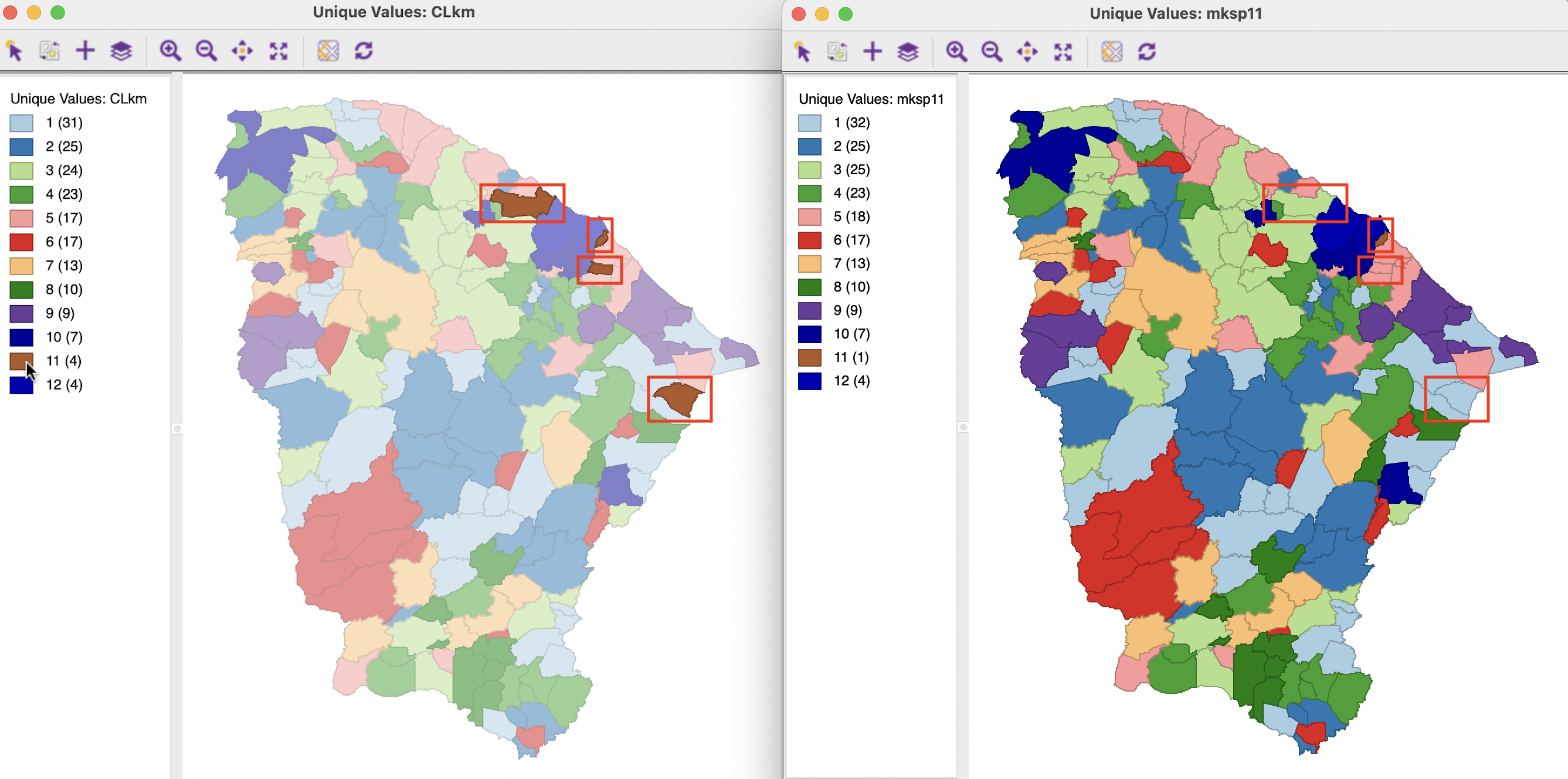
Figure 9.10: Make Spatial Cluster 11

The heuristic then moves to the next smallest cluster, C10, which consists of four disconnected parts: two singletons, one group of two municipalities, and one group of three, as shown in the red rectangles in the left-hand panel of Figure 9.11. The singletons are assigned to the largest adjoining units, respectively C3 for the top-most one, and C2 for the other one. The two entities in the north are assigned to C3. The remaining cluster of three units becomes the final cluster 10, as depicted in the right-hand panel.

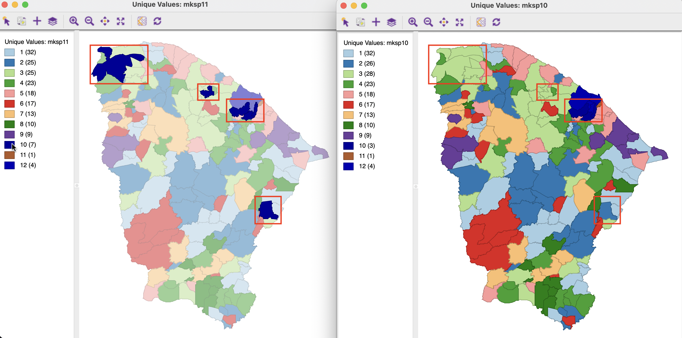
Figure 9.11: Make Spatial Cluster 10

The process continues until all unconnected entities are assigned.

9.5.1 Implementation

The heuristic can be started from the cluster toolbar icon as the item Make Spatial (in the very bottom part of the list), or alternatively as SC K Means. The latter is a bit of a misnomer, since it is not actually a spatially constrained K-Means algorithm, but rather the spatial post-processing of a K-Means solution. The SC K Means interface is the same as for regular K-Means, except that Spatial Weights need to be selected. In this case, the post-processing is part of the overall calculations and does not need to be carried out separately.

The Make Spatial Settings dialog has a slightly different look from the standard cluster interface. The main inputs are Select Cluster Indicator and the Cluster Variables. The cluster indicator is an integer variable that was saved as the output of a previous clustering exercise. The cluster variables are only included to compute the cluster characteristics at the end. They are not part of the actual heuristic. A Spatial Weights file needs to be specified as well (here, queen contiguity). In addition, there is the usual Transformation option, again to make sure the cluster characteristics are computed correctly.

The resulting cluster map for K-Means is shown in Figure 9.12. In contrast to the convention for unique values maps, the categories are not ordered by size, but they are kept in the same order as for the original cluster map. Consequently, the map in Figure 9.12 has the same cluster categories and colors as the map in Figure 9.10. The number of cluster elements in the final solution are given in parentheses next to the cluster category.

The spatial layout of the clusters shows little resemblance to the other (pseudo-)spatial solutions in this chapter because the centroid coordinates are not part of the heuristic. Instead, it is based on contiguity.

Figure 9.12: Make Spatial Cluster Map

Finally, the cluster characteristics are listed in Figure 9.13. Since the attributes are ignored in the spatial operations, the resulting within-cluster sum of squares are much worse. The overall BSS/TSS ratio is 0.285, similar (and slightly better) to the weighted optimization result.

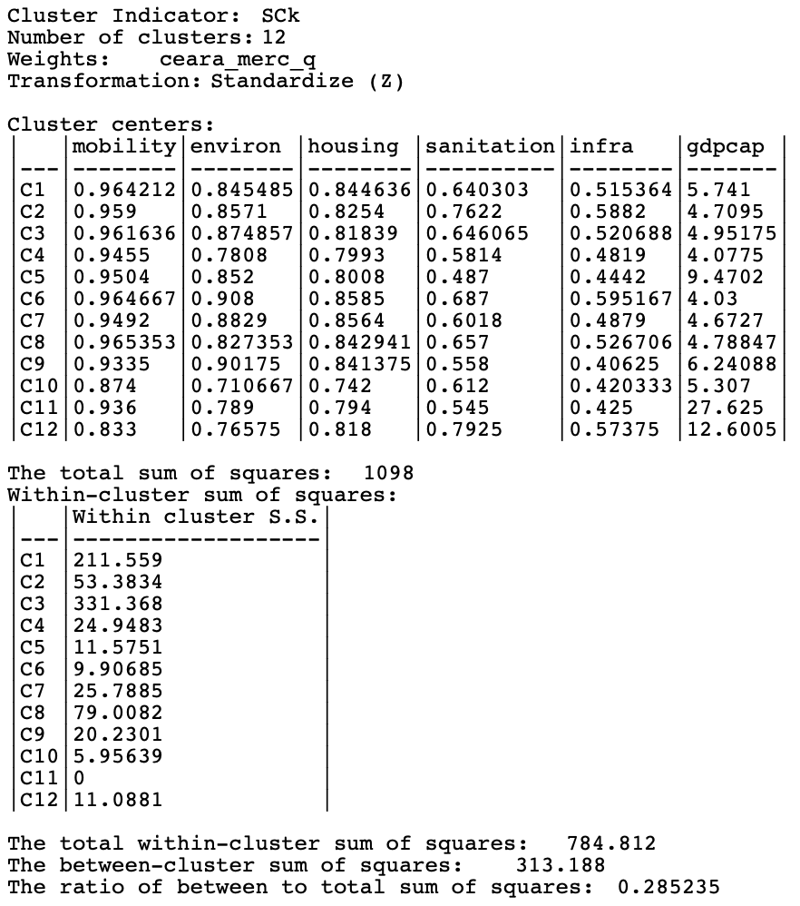
Figure 9.13: Make Spatial Cluster Characteristics

As mentioned, the approaches outlined in this chapter are primarily for pedagogical purposes, to illustrate the difficult trade offs between attribute and locational similarity. The results are seldom optimal, or even good, but they highlight the tension between the two objectives. In most applications, there is no easy solution that satisfies both goals.