5.3 Agglomerative Clustering

An agglomerative clustering algorithm starts with each observation serving as its own cluster, i.e., beginning with \(n\) clusters of size 1. Next, the algorithm moves through a sequence of steps, where each time the number of clusters is decreased by one, either by creating a new cluster by joining two individual observations, by assigning an observation to an existing cluster, or by merging two clusters. Such algorithms are sometimes referred to as SAHN, which stands for sequential, agglomerative, hierarchic and non-overlapping (Müllner 2011).

The sequence of merging observations into clusters is graphically represented by means of a tree structure, the so-call dendrogram (see Section 5.3.2). At the bottom of the tree, the individual observations constitute the leaves, whereas the root of the tree is the single cluster that consists of all observations.

The smallest within-group sum of squares is obtained in the initial stage, when each observation is its own cluster. As a result, the within sum of squares is zero and the between sum of squares is at its maximum, which also equals the total sum of squares. As soon as two observations are grouped, the within sum of squares increases. Hence, each time a new merger is carried out, the overall objective of minimizing the within sum of squares deteriorates. At the final stage, when all observations are joined into a single cluster, the total within sum of squares now also equals the total sum of squares, since there is no between sum of squares (the two are complementary).

In other words, in an agglomerative hierarchical clustering procedure, the objective function gets worse at each step. It is therefore not optimized as such, but instead can be evaluated at each step.

One distinguishing characteristic of hierarchical clustering is that once an observation is grouped with other observations, it cannot be disassociated from them in a later step. This precludes swapping of observations between clusters, which is a characteristic of some of the partitioning methods. This property of getting trapped into a cluster (i.e., into a branch of the dendrogram) can be limiting in some contexts.

5.3.1 Linkage and Updating Formula

A key aspect in the agglomerative process is how to define the distance between clusters, or between a single observation and a cluster. This is referred to as the linkage. There are at least seven different concepts of linkage, but here only the four most common ones are considered: single linkage, complete linkage, average linkage, and Ward’s method.

A second important concept is how the distances between other points (or clusters) and a newly merged cluster are computed, the so-called updating formula. With some clever algebra, it can be shown that these calculations can be based on the dissimilarity matrix from the previous step. The update thus does not require going back to the original \(n \times n\) dissimilarity matrix.²² Moreover, at each step, the dimension of the relevant dissimilarity matrix decreases by one, which allows for very memory-efficient algorithms.

Each linkage type and its associated updating formula is briefly considered in turn.

5.3.1.1 Single linkage

For single linkage, the relevant dissimilarity is between the two points in each cluster that are closest together. More precisely, the dissimilarity between clusters \(A\) and \(B\) is: \[d_{AB} = \mbox{min}_{i \in A,j \in B} d_{ij},\] The updating formula yields the dissimilarity between a point (or cluster) \(P\) and a cluster \(C\) that was obtained by merging \(A\) and \(B\). It is the smallest of the dissimilarities between \(P\) and \(A\) and \(P\) and \(B\): \[d_{PC} = \mbox{min}(d_{PA},d_{PB}).\] The minimum condition can also be obtained as the result of an algebraic expression, which yields the updating formula as: \[d_{PC} = (1/2) (d_{PA} + d_{PB}) - (1/2)| d_{PA} - d_{PB} |,\] in the same notation as before.²³

The updating formula only affects the row/column in the dissimilarity matrix that pertains to the newly merged cluster. The other elements of the dissimilarity matrix remain unchanged.

Single linkage clusters tend to result in a few clusters consisting of long drawn out chains of observations, in combination with several singletons (observations that form their own cluster). This is due to the fact that disparate clusters may be joined when they have two close points, but otherwise are far apart. Single linkage is sometimes used to detect outliers, i.e., observations that remain singletons and thus are far apart from all others.

5.3.1.2 Complete linkage

Complete linkage is the opposite of single linkage in that the dissimilarity between two clusters is defined as the farthest neighbors, i.e., the pair of points, one from each cluster, that are separated by the greatest dissimilarity. For the dissimilarity between clusters \(A\) and \(B\), this boils down to: \[d_{AB} = \mbox{max}_{i \in A,j \in B} d_{ij}.\] The updating formula is the opposite of the one for single linkage. The dissimilarity between a point (or cluster) \(P\) and a cluster \(C\) that was obtained by merging \(A\) and \(B\) is the largest of the dissimilarities between \(P\) and \(A\) and \(P\) and \(B\): \[d_{PC} = \mbox{max}(d_{PA},d_{PB}).\]

The algebraic counterpart of the updating formula is: \[d_{PC} = (1/2) (d_{PA} + d_{PB}) + (1/2)| d_{PA} - d_{PB} |,\] using the same logic as in the single linkage case.

In contrast to single linkage, complete linkage tends to result in a large number of well-balanced compact clusters. Instead of merging fairly disparate clusters that have (only) two close points, it can have the opposite effect of keeping similar observations in separate clusters.

5.3.1.3 Average linkage

In average linkage, the dissimilarity between two clusters is the average of all pairwise dissimilarities between observations \(i\) in cluster \(A\) and \(j\) in cluster \(B\). There are \(n_A.n_B\) such pairs (only counting each pair once), with \(n_A\) and \(n_B\) as the number of observations in each cluster. Consequently, the dissimilarity between \(A\) and \(B\) is (without double counting pairs in the numerator): \[d_{AB} = \frac{\sum_{i \in A} \sum_{j \in B} d_{ij}}{n_A.n_B}.\] In the special case when two single observations are merged, \(d_{AB}\) is simply the dissimilarity between the two, since \(n_A = n_B = 1\) and thus the denominator in the expression is 1.

The updating formula to compute the dissimilarity between a point (or cluster) \(P\) and the new cluster \(C\) formed by merging \(A\) and \(B\) is the weighted average of the dissimilarities \(d_{PA}\) and \(d_{PB}\): \[d_{PC} = \frac{n_A}{n_A + n_B} d_{PA} + \frac{n_B}{n_A + n_B} d_{PB}.\] As before, the other distances are not affected.²⁴

Average linkage can be viewed as a compromise between the nearest neighbor logic of single linkage and the furthest neighbor logic of complete linkage.

5.3.1.4 Ward’s method

The three linkage methods discussed so far only make use of a dissimilarity matrix. How this matrix is obtained does not matter. As a result, dissimilarity may be defined using Euclidean or Manhattan distance, dissimilarity among categories, or even directly from interview or survey data.

In contrast, the method developed by Ward (1963) is based on a sum of squared errors rationale that only works for Euclidean distance between observations. In addition, the sum of squared errors requires the consideration of the so-called centroid of each cluster, i.e., the mean vector of the observations belonging to the cluster. Therefore, the input into Ward’s method is not a dissimilarity matrix, but a \(n \times p\) matrix \(X\) of \(n\) observations on \(p\) variables (as before, this is typically standardized in some fashion).

Ward’s method is based on the objective of minimizing the deterioration in the overall within sum of squares. The latter is the sum of squared deviations between the observations in a cluster and the centroid (mean): \[WSS = \sum_{i \in C} (x_i - \bar{x}_C)^2,\]

with \(\bar{x}_C\) as the centroid of cluster \(C\).

Since any merger of two existing clusters (including the merger of individual observations) results in a worsening of the overall WSS, Ward’s method is designed to minimize this deterioration. More specifically, it is designed to minimize the difference between the new (larger) WSS in the merged cluster and the sum of the WSS of the components that were merged. This turns out to boil down to minimizing the distance between cluster centers.²⁵ Without loss of generality, it is easier to express the dissimilarity in terms of the square of the Euclidean distance: \[d_{AB}^2 = \frac{2n_A n_B}{n_A + n_B} ||\bar{x}_A - \bar{x}_B ||^2,\] where \(||\bar{x}_A - \bar{x}_B ||\) is the Euclidean distance between the two cluster centers (squared in the distance squared expression).²⁶

The update equation to compute the (squared) distance from an observation (or cluster) \(P\) to a new cluster \(C\) obtained from the merger of \(A\) and \(B\) is more complex than for the other linkage options: \[d^2_{PC} = \frac{n_A + n_P}{n_C + n_P} d^2_{PA} + \frac{n_B + n_P}{n_C + n_P} d^2_{PB} - \frac{n_P}{n_C + n_P} d^2_{AB},\] in the same notation as before. However, it can still readily be obtained from the information contained in the dissimilarity matrix from the previous step, and it does not involve the actual computation of centroids.

To see why this is the case, consider the usual first step when two single observations are merged. The distance squared between them is simply the Euclidean distance squared between their values, not involving any centroids. The updated squared distances between other points and the two merged points only involve the point-to-point squared distances \(d^2_{PA}\), \(d^2_{PB}\) and \(d^2_{AB}\), no centroids. From then on, any update uses the results from the previous distance matrix in the update equation.

5.3.1.5 Illustration - single linkage

To illustrate the logic of agglomerative hierarchical clustering algorithms, the single linkage approach is applied to a toy example consisting of the coordinates of seven points, shown in Figure 5.2. The corresponding X, Y values are listed in Figure 5.3. The point IDs are ordered with increasing values of X first, then Y, starting with observation 1 in the lower left corner.

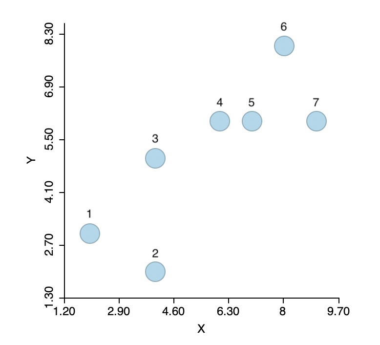
Figure 5.2: Single linkage hierarchical clustering toy example

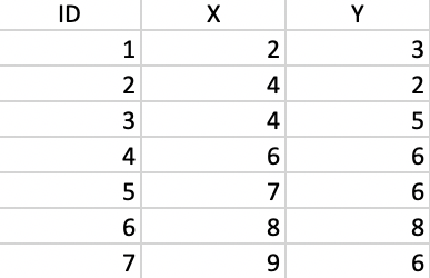
Figure 5.3: Coordinate Values

The basis for any agglomerative clustering method is a \(n \times n\) symmetric dissimilarity matrix. Except for Ward’s method, this is the only information needed. The dissimilarity matrix derived from the Euclidean distances between the points is shown in Figure 5.4. Since the matrix is symmetric, only the upper diagonal elements are listed.

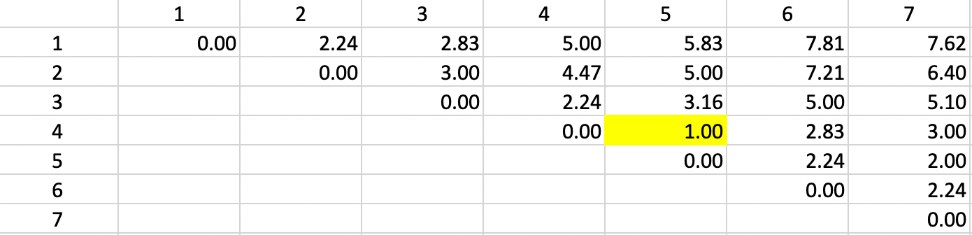
Figure 5.4: Single Linkage - Step 1

The first step in the algorithm is to identify the pair of observations that have the smallest nearest neighbor distance. In the distance matrix, this is the row-column combination with the smallest entry. In Figure 5.4 this is readily identified as the pair 4-5 (\(d_{4,5}=1.0\)). This pair therefore forms the first cluster, connected by a link in Figure 5.5. The two points in the cluster are highlighted in dark blue. The five other observations remain in their initial separate cluster. In other words, at this stage, there are six clusters, one less than the number of observations.

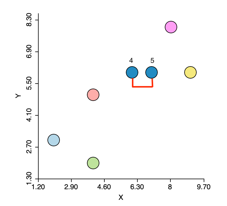
Figure 5.5: Smallest nearest neighbors

The dissimilarity matrix is updated using the smallest dissimilarity between each observation and either observation 4 or observation 5. This yields the updated row and column entries for the combined unit 4,5. More precisely, the dissimilarity used between the cluster and the other observations varies depending on whether observation 4 or 5 is closest to the other observations. For example, in Figure 5.6, the dissimilarity between 4,5 and 1 is given as 5.0, which is the smallest of 1-4 (5.0) and 1-5 (5.83). The dissimilarities between the pairs of observations that do not involve 4,5 are not affected.

The other entries for 4,5 are updated in the same way, and again the smallest dissimilarity is located in the matrix. This time, it is a dissimilarity of 2.0 between 4,5 and 7 (more precisely, between the closest pair 5 and 7). Consequently, observation 7 is added to the 4,5 cluster.

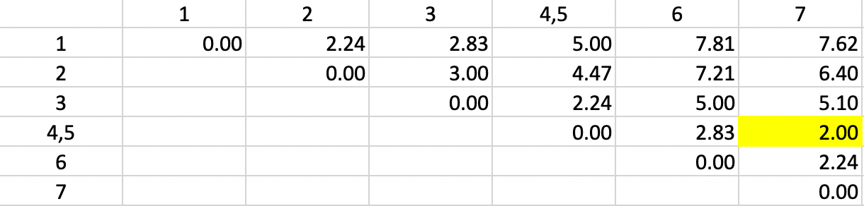
Figure 5.6: Single Linkage - Step 2

The dissimilarities between 4,5,7 and the other points are updated in Figure 5.7. However, now there is a problem. There is a three-way tie in terms of the smallest value: 1-2, 4,5,7-3 and 4,5,7-6 all have a dissimilarity of 2.24, but only one can be picked to update the clusters. Ties are typically handled by choosing one grouping at random. In the example, the pair 1-2 is selected, which is how the tie is broken by the algorithm used in GeoDa.²⁷

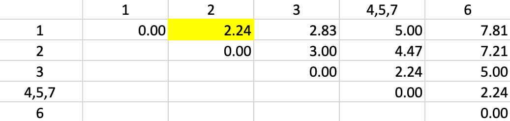
Figure 5.7: Single Linkage - Step 3

With the distances updated, not unsurprisingly, 2.24 is again found as the shortest dissimilarity, tied for two pairs (in Figure 5.8). This time the algorithm adds 3 to the existing cluster 4,5,7.

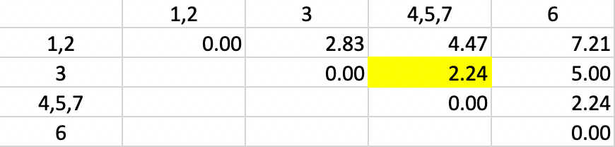
Figure 5.8: Single Linkage - Step 4

Finally, observation 6 is added to cluster 4,5,7,3 again for a dissimilarity of 2.24 (in Figure 5.9).

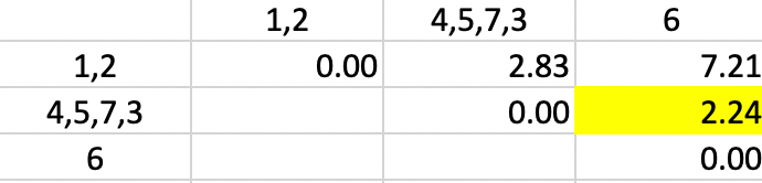
Figure 5.9: Single Linkage - Step 5

The end result is to merge the two clusters 1-2 and 4,5,7,3,6 into a single one, which ends the iterations (Figure 5.10).

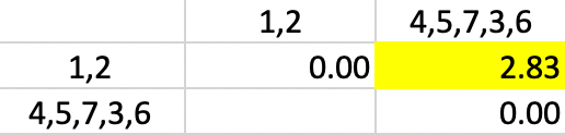
Figure 5.10: Single Linkage - Step 6

In sum, the algorithm moves sequentially to identify the nearest neighbor at each step, merges the relevant observations/clusters and so decreases the number of clusters by one. The sequence of steps is illustrated in the panels of Figure 5.11, going from left to right and starting at the top.

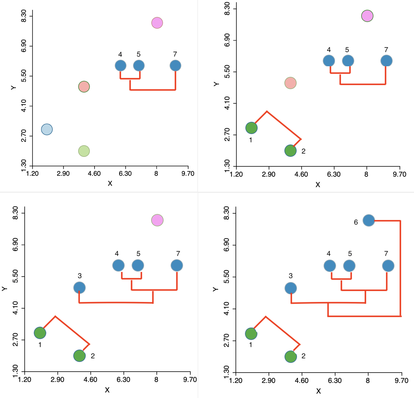
Figure 5.11: Single linkage iterations

5.3.2 Dendrogram

While the visual representation of the sequential grouping of observations in Figure 5.11 works well in this toy example, it is not practical for larger data sets.

A tree structure that visualizes the agglomerative nesting of observations into clusters is the so-called dendrogram. For each step in the process, the graph shows which observations/clusters are combined. In addition, the degree of change in the objective function achieved by each merger is visualized by a corresponding distance on the horizontal (or vertical) axis.

The implementation of the dendrogram in GeoDa is currently somewhat limited, but it accomplishes the main goal. In Figure 5.12, the dendrogram is illustrated for the single linkage method in the toy example. The graph shows how the cluster starts by combining two observations (4 and 5), to which then a third (7) is added. These first two steps are contained inside the highlighted black square in the figure. The corresponding observations are selected as entries in a matching data table.

Next, following the tree structure reveals how two more observations (1 and 2) are combined into a separate cluster, and two observations (3 and 6) are added to the original cluster of 4,5 and 7. Given the three-way tie in the inter-group distances, the last three operations all line up (same distance from the right side) in the graph. As a result, the change in the objective function (more precisely, a deterioration) that follows from adding the points to a cluster is the same in each case.

The dashed vertical line represents a cut line. It corresponds with a particular value of k for which the make up of the clusters and their characteristics can be further investigated. As the cut line is moved, the members of each cluster are revealed that correspond with a different value for \(k\).

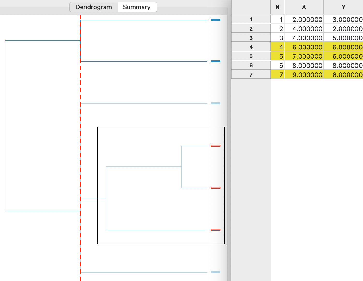
Figure 5.12: Single linkage dendrogram

In practice, important cluster characteristics are computed for each of the selected cut points, such as the sum of squares, the total within sum of squares, the total between sum of squares, and the ratio of the the total between sum of squares to the total sum of squares (the higher ratio, the better). This will be further illustrated as part of the discussion of implementation issues in the next section.

---

22. Detailed proofs for all the properties are contained in Chapter 5 of Kaufman and Rousseeuw (2005).↩︎

23. To see that this holds, consider the situation when \(d_{PA} < d_{PB}\), i.e., \(A\) is the nearest neighbor to \(P\). As a result, the absolute value of \(d_{PA} - d_{PB}\) is \(d_{PB} - d_{PA}\). Then the expression becomes \((1/2) d_{PA} + (1/2) d_{PB} - (1/2) d_{PB} + (1/2) d_{PA} = d_{PA}\), the desired result.↩︎

24. By convention, the diagonal dissimilarity for the newly merged cluster is set to zero.↩︎

25. See Kaufman and Rousseeuw (2005), Chapter 5, for detailed proofs.↩︎

26. The factor 2 is included to make sure the expression works when two single observations are merged. In such an instance, their centroid is their actual value and \(n_A + n_B = 2\). It does not matter in terms of the algorithm steps.↩︎

27. An implementation of the fastcluster algorithm.↩︎