3.5 Spatializing MDS
A distinct aspect of the treatment of multi-dimensional scaling in this book, and a perspective largely absent in the rest of the literature, is a focus on spatializing the results. More precisely, several approaches are described that allow to investigate a closer link between distance in attribute space and distance in geographical space. This provides an alternative way to approach the problem of multivariate spatial clustering, in which the explicit multivariate aspect is sidestepped by exploiting the relative locations in the MDS scatter plot.
The points in the MDS scatter plot can be viewed as locations in a two-dimensional attribute space. This is an example of the use of geographical concepts (location, distance) in contexts where the space is non-geographical. It also allows a further investigation and visualization of the tension between attribute similarity and locational similarity, two core components underlying the notion of spatial autocorrelation.
An explicit spatial perspective is introduced by linking the MDS scatter plot with various map views of the data. In addition, it is possible to exploit the location of the points in attribute space to construct spatial weights based on neighbors in the MDS plot. These weights can then be compared to their geographical counterparts to discover overlap. Furthermore, the point locations themselves can be incorporated in a cluster analysis.
The obvious connection between the MDS scatter plot and a map is explored first, through linking and brushing. Next, the focus shifts to the use of the spatial weights concept to formalize the neighbor structure obtained in the solution of MDS. This is further explored through an alternative to the local neighbor match test of Chapter 18 in Volume 1, based on the k-nearest neighbor structure in the MDS scatter plot. Finally, the application to point locations in the MDS of density based cluster methods from Chapter 20 in Volume 1 is considered as well.
3.5.1 MDS and Map
An example of linking observations between the MDS scatter plot and a map was given in Figure 3.12, where a subset of observations from the scatter plot was also shown on a map. Instead of using locations only, as in the point map in Figure 3.12, one can also link and brush a thematic map. For example, in Algeri et al. (2022), the bank efficiency indicators are related to an overall technical output efficiency measure.15 Linking a thematic map for this variable to the MDS scatter plot provides insight into the match of patterns in the map for this dependent variable and interesting groupings of the explanatory variable in the MDS scatter plot.
Other maps can be linked as well. For example, Figure 3.15 shows a Local Moran cluster map for the technical output efficiency variable, TE_OUT(2013) (based on queen contiguity, 99,999 permutations and p < 0.01) linked to the MDS scatter plot for SMACOF, using Euclidean distance (the same as Figure 3.8). The observations in the High-High clusters are selected on the left, and their corresponding points in the MDS space for the explanatory variables highlighted on the right. While several cluster locations have closely aligned points in the MDS, for others this is not the case at all. A careful brushing of the map (and/or other maps) can shed further light on the degree of agreement of the two concepts of clustering.
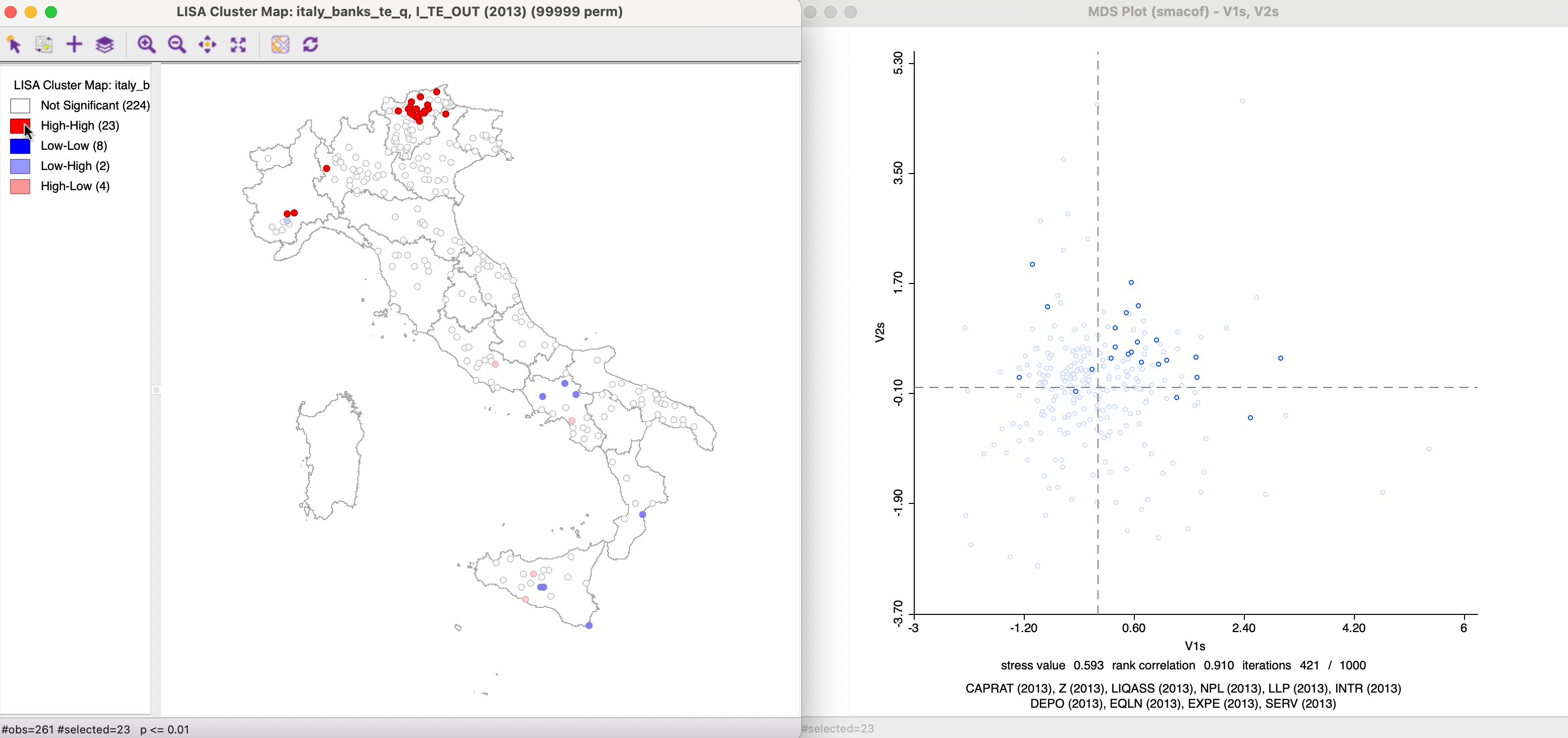
Figure 3.15: Linked Local Moran Cluster Map and MDS
3.5.2 MDS Spatial Weights
As mentioned, the points in the MDS scatter plot can be viewed as locations in an embedded attribute space. As such, they can be mapped. In such a point map, the neighbor structure among the points can be exploited to create spatial weights, in exactly the same way as for geographic points (e.g., the distance bands, k-nearest neighbors, contiguity from Thiessen polygons considered in Chapter 11 of Volume 1. Conceptually, such spatial weights are similar to the distance weights created from multiple variables, but they are based on inter-observation distances from an embedded high-dimensional object in two dimensions. While this involves some loss of information, the associated two-dimensional visualization is highly intuitive.
In GeoDa, there are three ways to create spatial weights from points in a MDS scatter plot. One is to explicitly create a point layer using the MDS coordinates (for example, V1s and V2s), by means of Tools > Shape > Points from Table. Once the point layer is in place, the standard spatial weights functionality can be invoked.
A second way pertains only to distance weights. It again uses the Weights Manager, but with the Variables option for Distance Weight, and by specifying the MDS coordinates as the variables. This limits the weights to distance band and k-nearest neighbors. Since these coordinates are already normalized in a way, the Raw setting is appropriate for standardization.
A final method applies directly to the MDS scatterplot. A right click in the plot reveals Create Weights as the top option.
This brings up the standard Weights File Creation interface. The difference with the previous approach is that the MDS coordinates do not need to be specified, but are taken directly from the MDS scatter plot where the option is invoked. In addition, it is also possible to create contiguity weights from the Thiessen polygons associated with the scatter plot points.
3.5.2.1 Attribute and geographical neighbors
An obvious comparison of attribute and geographical similarity is to investigate the extent to which the k-nearest neighbors in geographic space match neighbors in attribute space using the Intersection functionality in the Weights Manager.
For example, k-nearest neighbor weights for k=6 and using the SMACOF Euclidean distance can be created using one of the three methods just outlined (i.e., based on V1s and V2s as the coordinate values). These k-nearest neighbor weights can be intersected with their geographic k-nearest neighbor counterparts (e.g., the file italy_banks_te_k6.gwt created in Chapter Chapter 11 of Volume 1). This results in a gal weights file that lists for each observation the neighbors that are shared between the two k-nearest neighbor files.
As is to be expected, the resulting file is much sparser than the original weights. The associated Connectivity Histogram, reveals that 21 observations have 2 matches, 67 observations have one match, and the remaining 173 observations have no match.
The Save Connectivity to Table option can be used to create a variable that reflects this cardinality. Such a variable then lends itself to a Unique Values Map, as shown in the left-hand panel of Figure 3.16. The observations with 2 matches are linked to the corresponding points in the MDS scatter plot. This reveals how several of the close neighbors in space are also close neighbors in multi-attribute space, suggesting the presence of multivariate spatial clustering.
This is pursued more formally by means of the Local Neighbor Match Test in Section 3.5.3.
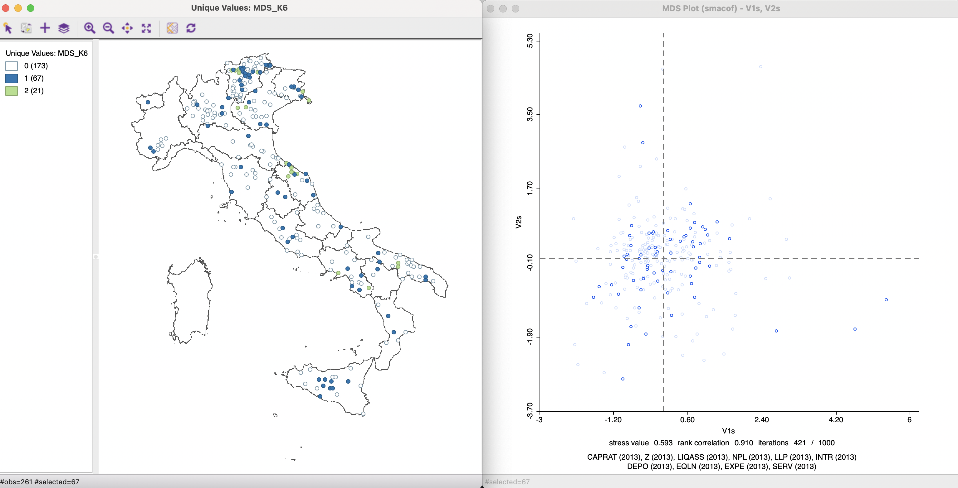
Figure 3.16: Common Connectivity K-6 Neighbors
3.5.2.2 Common coverage percentage
The Intersection functionality for spatial weights can also be employed to compare the nearest neighbor structures implied by different MDS solutions, both with respect to the geographical counterpart as well as for the overlapping neighbor structures between them.
One indication of a different degree of match between attribute and geographical similarity is to compare the percentage non-zero weights in the overlap to the maximum, based on k neighbors for each observation. In the current example, the percent non-zero weights for the base result is 2.30%. A perfect match between attribute neighbors and geographic neighbors would therefor yield a ratio of 100%. Various non-spatial weights can be compared to the spatial counterpart by computing the ratio of non-zero weights for the intersection to the maximum possible. This metric can then be referred to as the common coverage percentage.
A comparison of the three MDS solutions in terms of overlap with corresponding geographical neighbors yields 0.14% non-zero for the classic metric solution, 0.16% for the SMACOF solution with Euclidean weights, and 0.16% for SMACOF with Manhattan distance. This yields common coverage percentages of respectively 6.09% and 6.96%, showing very similar (low) overlap with spatial neighbors.
This same approach can also be employed to assess the commonality between k-nearest neighbor graphs constructed for different sets of MDS coordinates. In the example, the common coverage percentage is 1.07/2.30, or 46.5% between classic metric and Euclidean SMACOF, 0.08/2.30, or 3.48% between classic metric and Manhattan SMACOF, and 1.40/2.30, or 60.87% between the two SMACOF distance metrics. This approach provides a more quantitative assessment of match between MDS solutions than a visual inspection of the MDS scatter plot and highlights the important differences between classic metric and SMACOF using the Manhattan metric.
3.5.3 MDS Neighbor Match Test
A final, more formal approach to check the similarity between neighbors in attribute space and neighbors in geographic space is to consider it as a special case of the local neighbor match test. Instead of using the k-nearest neighbor relation for the high-dimensional space, the same relation can be used in the two- or three-dimensional MDS space.
The accomplish this, the MDS coordinates are selected as the variables in the interface for Space > Local Neighbor Match Test (see Chapter 11 of Volume 1). For example, this can be applied to the same V1s and V2s coordinates as before. As usual, an option is provided to save the cardinality of the weights intersection between the attribute knn weights and the geographical knn weights, as well as the associated probability of finding that many neighbors in common.
The associated unique values map with the common connection shown as a graph is given in Figure 3.17, which, except for the connections, is identical to the left-hand panel in Figure 3.16.
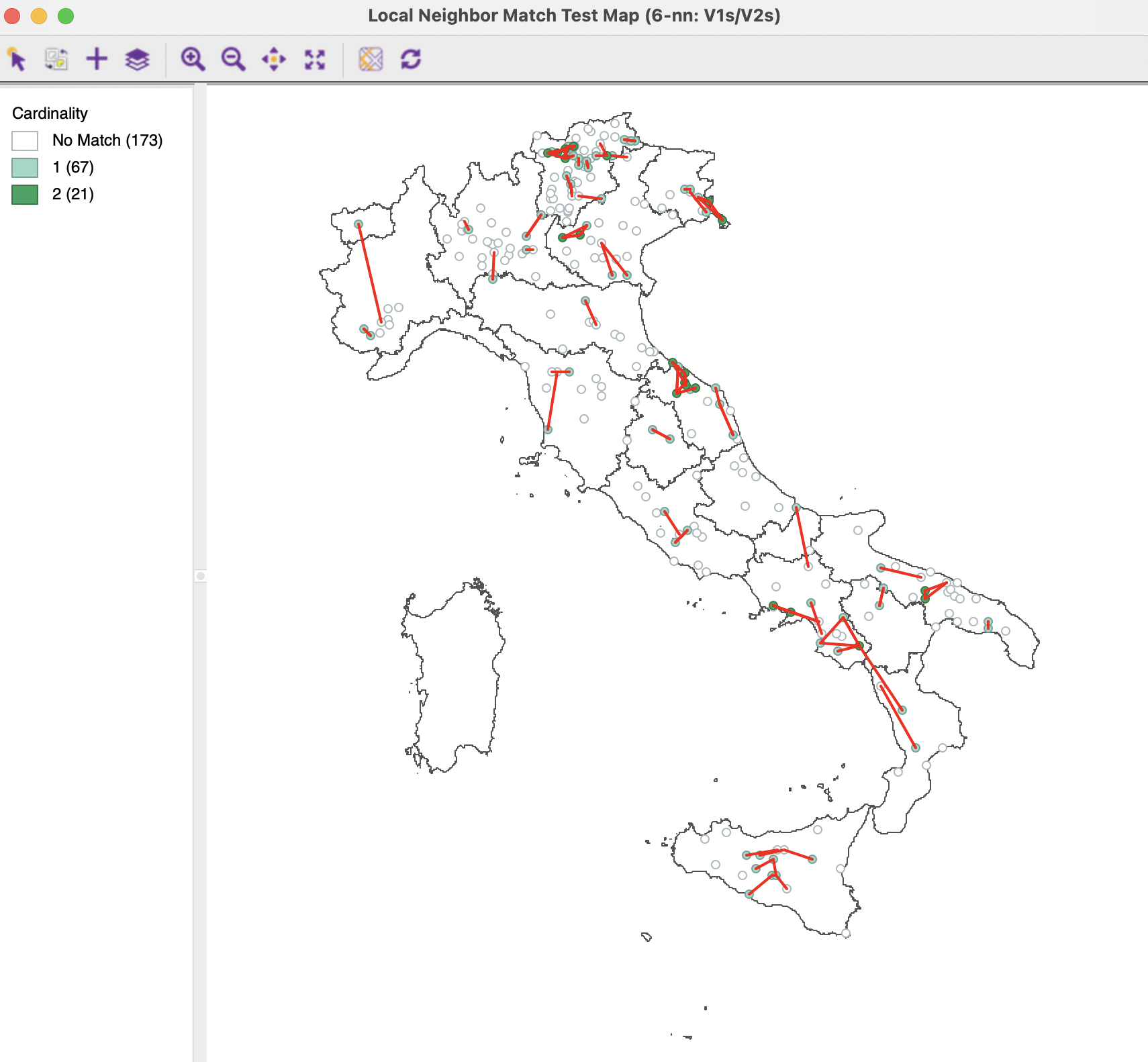
Figure 3.17: Local Neighbor Match Test for MDS
The cpval column in the data table reveals that locations with two matches have an associated \(p\)-value of 0.0062. However, the \(p\)-value associated with one common match is only 0.13, which cannot be deemed to be significant.
These results can be compared to a multivariate Local Neighbor Match Test applied to all ten variables. Figure 3.18 shows the results for the latter. Relative to classic MDS, there are more matches for the full multi-attribute result, with six observations achieving three common neighbors (p=0.000133), in addition to 18 with two neighbors and 82 with one neighbor.
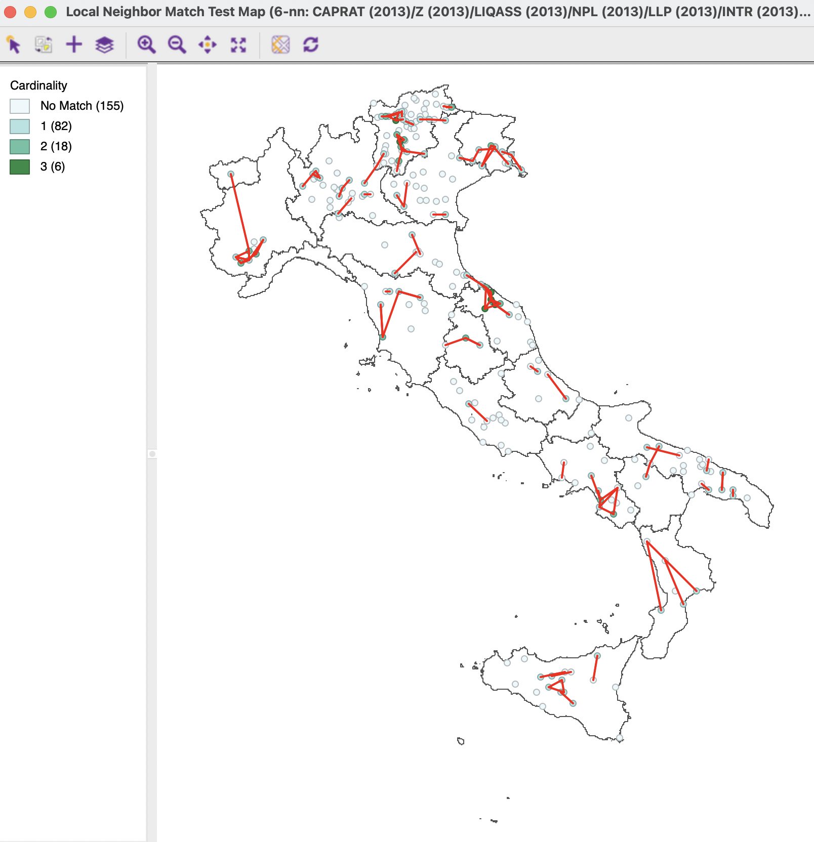
Figure 3.18: Multivariate Local Neighbor Match Test
An advantage of using the coordinates in embedded space is that the curse of dimensionality is avoided. Instead of having to compute k-nearest neighbors in high dimensions, the MDS results are limited to two or three dimensions, which is computationally easy. In the current example, the trade-off seems to be that MDS results in fewer highly significant clusters.
3.5.4 HDBSCAN and MDS
A final spatial perspective on the MDS results considered here is the application of density based clustering methods to the MDS coordinate points. This operates in the standard way, as described in Chapter 20 of Volume 1. The clustering routines identify subsets of points in the MDS scatter plot that are close together. Indirectly, this provides a way to cluster in multi-attribute space.
Because the density based clustering results are linked to a map, the extent of geographic association between the cluster points is visualized as well. For example, the right-hand panel of Figure 3.19 shows the outcome of an HDBSCAN routine on the coordinates V1s and V2s, with a minimum cluster size of 7. This yields three clusters, containing respectively 54, 13 and 8 observations, depicted in the map. As in the previous analyses, there is some degree of overlap between geographic neighbors and MDS neighbors, but many MDS neighbors are also not geographically close.
The left-hand panel of Figure 3.19 identifies the three clusters on the MDS scatter plot. This figure is created as a bubble chart for a categorical variable, with the cluster category as the variable associated with the bubble color. The three groupings of points are clearly delineated.
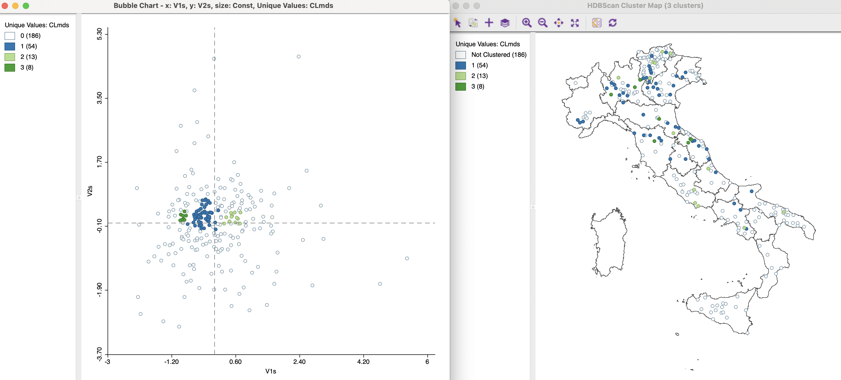
Figure 3.19: HDBSCAN for MDS
The methods outlined in this section provide several alternatives to a full multivariate clustering exercise by means of the summary information contained in the MDS results. In some instances they may alleviate problems associated with the curse of dimensionality. Together with graphs such as a parallel coordinate plot, further insight can be gained into the relative contribution of variables to the cluster results. By using a combination of these methods, interesting locations can be identified and further investigated by means of a careful sensitivity analysis.